Data Structures in C#

Rod Howell
Dept. of Computer Science
Kansas State University
Manhattan, KS 66506
USA

Email: rhowell@ksu.edu

This text is supplemental material for CIS 300 at Kansas State University. Its purpose is to provide a written summary of the material covered, with additional explanation and code examples beyond what are presented in class. A background of programming in Java is assumed, and an appendix summarizing some of the syntax of C# is provided. Because CIS 300 is a lab class, no attempt is made here to provide examples for all of the topics covered; instead, students are expected to provide many of their own examples through the lab exercises (in most cases, solutions to these exercises will be provided to enrolled students following the lab).

We assume the use of Visual Studio® Community 2022 . All examples, as well as all assignments in CIS 300, use .NET 6 and version 10 of the C# language. All graphical applications use Windows Forms (Windows Desktop 6 ).

Please send to Rod Howell any corrections, including typographical errors, missing images, and broken links.

Subsections of

Input/Output

Input and output are central concepts to computing - in order to be able to accomplish a computational task, a program must typically process some input and produce some output. Input and output may be presented in a variety of ways. For example, many programs communicate with users through a graphical user interface, or GUI. In the simplest case, the user performs some action, such as clicking the mouse on a button, thus signaling an event. A method in the program then responds to that event by reading information that the user has typed into various controls on the GUI, and processes that information. It may then provide output to the user by writing results to various controls on the GUI.

Such a simple presentation of input/output (or I/O) is far too limiting, however. For example, other mechanisms such as dialogs - secondary windows designed for exchanging specific information - may be used to avoid cluttering the main window. In other cases, the amount of data that needs to be exchanged is too large to be transferred through a GUI. In such cases, the program may need to read and/or write a file. This chapter addresses these more advanced I/O mechanisms.

Subsections of Input/Output

Dialogs

Dialogs are windows displayed by a program for the purpose of exchanging specific information with the user. There are two kinds of dialogs:

  • Modal dialogs block all other interaction with the program until the dialog is closed.
  • Non-modal dialogs allow the user to interact with the program in other ways while the dialog is open.

We will examine three classes provided by Microsoft® .NET 6, each of which implements a modal dialog. .NET provides various other classes, such as FolderBrowserDialog , FontDialog , and ColorDialog , that also implement specific kinds of dialogs. We conclude by discussing how custom dialogs may be built using Visual Studio®.

Subsections of Dialogs

Message Boxes

The MessageBox class (found in the System.Windows.Forms namespace) provides a simple mechanism for displaying a message and obtaining one of a few simple responses from the user. The most common usage of a MessageBox is to call one of its various Show methods, each of which is static . The simplest Show method takes a string as its only parameter. The method then displays this string in a modal dialog containing an “OK” button. Thus, for example,

MessageBox.Show("Hello world!");

will display the following dialog:

A MessageBox.

Because the dialog is modal, it will block all other interaction with the program until the user closes it by clicking either the “OK” button or the “X” in the upper right. Furthermore, the Show method will not return until that time.

Other Show methods allow greater customization of a MessageBox. For example, one Show method takes as an additional parameter a second string giving a caption for the MessageBox. Thus, the statement,

MessageBox.Show("Hello world!", "Hello");

will display the following modal dialog:

A MessageBox with a caption.

Other Show methods allow the buttons to be customized. For example, one Show method takes, as its third parameter, an element from the MessageBoxButtons enumeration . This enumeration contains the following values:

  • MessageBoxButtons.AbortRetryIgnore: Buttons labeled “Abort”, “Retry”, and “Ignore” are shown.
  • MessageBoxButtons.CancelTryContinue: Buttons labeled “Cancel”, “Try Again”, and “Continue” are shown.
  • MessageBoxButtons.OK: A single button labeled “OK” is shown.
  • MessageBoxButtons.OKCancel: Buttons labeled “OK” and “Cancel” are shown.
  • MessageBoxButtons.RetryCancel: Buttons labeled “Retry” and “Cancel” are shown.
  • MessageBoxButtons.YesNo: Buttons labeled “Yes” and “No” are shown.
  • MessageBoxButtons.YesNoCancel: Buttons labeled “Yes”, “No”, and “Cancel” are shown.

The values above containing the word, “Cancel”, cause the “X” in the upper-right of the dialog to be enabled. Clicking this button in these cases is equivalent to clicking the “Cancel” button. The value, MessageBoxButtons.OK, also enables this “X” button, but in this case, clicking this button is equivalent to clicking the “OK” button. Using a Show without a MessageBoxButtons parameter also gives this behavior. For all other MessageBoxButtons values, this “X” button is disabled.

In order to provide appropriate functionality to each of the buttons, each Show method returns a value of type DialogResult . This type is another enumeration containing the following values to indicate which button the user clicked:

  • DialogResult.Abort
  • DialogResult.Cancel
  • DialogResult.Continue
  • DialogResult.Ignore
  • DialogResult.No
  • DialogResult.None (this value won’t be returned by any of the Show methods)
  • DialogResult.OK
  • DialogResult.Retry
  • DialogResult.TryAgain
  • DialogResult.Yes

Suppose, for example, that we are writing a document formatter or some other application in which the user builds a document. If the user attempts to exit the program when the document is unsaved, we would like to give an opportunity to save the document. We can accomplish this with the following code:

DialogResult result = MessageBox.Show("The file is not saved. Really quit?", "Confirm Quit", MessageBoxButtons.YesNo);
if (result == DialogResult.Yes)
{
    Application.Exit();
}

The first statement displays the following dialog:

A MessageBox with Yes and No buttons

Again, because the dialog is modal, the Show method does not return until the user closes the dialog by clicking one of the two buttons (the “X” in the upper right is disabled). When the user does this, the dialog closes, and the Show method returns either DialogResult.Yes or DialogResult.No to indicate which button the user clicked. If the user clicked the “Yes” button, then the if-statement will cause the program to terminate. Otherwise, the program will continue with whatever code follows (probably nothing more, as the program will need to await further user action).

We can also decorate a MessageBox with an icon that indicates what type of message it is. This requires another Show method having a fourth parameter of type MessageBoxIcon . MessageBoxIcon is another enumeration. Some of its values are:

  • MessageBoxIcon.Error: A picture of an error icon should appear here. A picture of an error icon should appear here.
  • MessageBoxIcon.Information: A picture of an information icon should appear here. A picture of an information icon should appear here.
  • MessageBoxIcon.None (no icon)
  • MessageBoxIcon.Warning: A picture of a warning icon should appear here. A picture of a warning icon should appear here.

This enumeration contains a few other values as well, but they currently are simply duplicate values for the above icons or values that Microsoft recommends against using. To add a warning icon to the above example, we could replace the first statement with:

DialogResult result = MessageBox.Show("The file is not saved. Really quit?", "Confirm Quit", MessageBoxButtons.YesNo, MessageBoxIcon.Warning);

This will display the following dialog:

A MessageBox with an icon.

Notice that in the above example, the “Yes” button has the focus; i.e., pressing “Enter” has the same effect as clicking this button. It is usually desirable to have the safest response as the default - in this case, the “No” button. To achieve this, a Show method having a fifth parameter, of type MessageBoxDefaultButton , is required. MessageBoxDefaultButton is another enumeration having the following values to select an appropriate button to be the default:

  • MessageBoxDefaultButton.Button1
  • MessageBoxDefaultButton.Button2
  • MessageBoxDefaultButton.Button3
  • MessageBoxDefaultButton.Button4

Thus, the following statement:

DialogResult result = MessageBox.Show("The file is not saved. Really quit?", 
    "Confirm Quit", MessageBoxButtons.YesNo, MessageBoxIcon.Warning,
    MessageBoxDefaultButton.Button2);

produces a dialog similar to the one above, but having the “No” button as its default.

There are other Show methods that allow additional fine-tuning; however, the ones described here cover most of the functionality. For details on other Show methods, see the documentation for the MessageBox class .

File Dialogs

The System.Windows.Forms namespace contains two other classes that implement modal dialogs for obtaining file names from the user. These classes are OpenFileDialog , which is designed to obtain the name of a file to read, and SaveFileDialog , which is designed to obtain the name of a file to write. Because we often need to obtain the name of a file prior to doing file I/O, it is appropriate to consider these classes now.

Although these dialogs are visually separate from the window from which they are opened, it is possible (and usually desirable) to add instances of these classes to a form from the Design window . Both can be found in the “Dialogs” section of the Toolbox. They can be added to the form simply by double-clicking on their names. They will not appear on the form itself, but in a separate area of the Design window. Their properties can then be modified in the same way as any other control. We will discuss some of these properties a bit later in what follows.

Each of these classes has a method called ShowDialog that takes no parameters. For example, if we call the ShowDialog method of an OpenFileDialog, a dialog resembling the following will be opened:

An OpenFileDialog.

Similarly, calling the ShowDialog method of a SaveFileDialog opens a dialog resembling the following:

A SaveFileDialog.

Because these dialogs are modal, the method call will not return until the user closes the dialog. It will then return a DialogResult indicating how the user closed the form - either DialogResult.OK or DialogResult.Cancel (see the previous section for more information on the DialogResult type). Therefore, if uxFileDialog is a variable referring to a file dialog, we typically use the following code template to display it:

if (uxFileDialog.ShowDialog() == DialogResult.OK)
{
    // Process the file
}

Thus, if the user selects a file, we process it; otherwise, we do nothing. In some cases, we might include an else containing code that needs to be executed if the user closes the dialog without selecting a file.

Processing a file will be discussed in the three sections that follow. However, one thing we will certainly want to do prior to processing the file is to obtain the file name that the user selected (after all, this is the reason we display a file dialog). We can obtain this file name via the dialog’s FileName property ; for example,

string fileName = uxFileDialog.FileName;

Note that this and other properties are accessible for initialization purposes through a file dialog’s Properties window in the Designer. This is useful for an OpenFileDialog’s FileName property, as the default supplied by Visual Studio® is rather odd. Other properties that we might want to initialize here (in addition to (Name), the name of the variable referring to the dialog) include:

  • Title , the title of the dialog (by default, “Open” for an OpenFileDialog or “Save As” for a SaveFileDialog).

  • Filter , a filter string, which controls what file types will be displayed. An example of a filter string is: C# files|*.cs|All files|*.*. A filter string consists of an even number of components separated by vertical bars ("|"). Thus, the above filter string consists of four components. These components are grouped into pairs. The first component of each pair gives the string that will be displayed in the dialog to describe what files are displayed. The second component of each pair describes a pattern of file names to be displayed when the first component of that pair is shown. Use an asterisk ("*") in a pattern to denote any sequence of characters. The “.” in a pattern ending in “.*” does not need to be matched - a file without an extension will be listed if it matches the pattern to the left of the “.”. Multiple patterns, separated by semicolons (";"), may be listed in one component. Thus, the above filter string describes two filters that the user may choose from. The first filter is labeled, “C# files”, and lists all files ending in “.cs”. The second filter is labeled “All files”, and lists all files.

  • FilterIndex indicates which pair in the filter string is currently being used. Note that the first pair has an index of 1, not 0.

  • AddExtension and DefaultExt control the dialog’s behavior when the user types in a file name without an extension. When this happens, if a filter with a unique extension is chosen, that extension will be appended, regardless of the values of these two properties. Otherwise, if AddExtension is True, the value of DefaultExt will be appended, following a “.”.

Other properties allow further customization of file dialogs. For more details, see the OpenFileDialog and SaveFileDialog documentation.

Custom Dialogs

While the dialogs provided by the .NET Framework are useful in a variety of applications, there are times when we need to be able to design our own special-purpose dialog to obtain specific information from the user. This section outlines how Visual Studio® can be used to build such a dialog.

Let’s begin by considering a simple example. Suppose we are building an application that needs a dialog to obtain from the user the following pieces of information:

  • a name;
  • a phone number; and
  • a number of siblings.

In order to keep the example simple, the program will simply display this information in its main window. Thus, the main window looks like this:

A GUI displaying a person's information.

Clicking the “Get New Information” button will open our custom dialog, which will look like this:

A custom dialog.

After the user enters the information, clicking “OK” will cause the information entered to be displayed in the main window. If the user clicks “Cancel”, the main window will be unchanged.

After building the main form in Visual Studio’s Design Window, we can build the dialog by creating another form. To do this, in the Solution Explorer, right-click on the project name and select “Add->Form (Windows Forms)…”. This will open a dialog for adding a new item, where the type of item is pre-selected to be a Windows Form. You will need to supply a name for the form. This name will serve as both a file name for a source file and the name of a class defined within this file. For example, we could choose the name, “InformationDialog.cs”, and the class will be named InformationDialog. Clicking the “Add” button will then open a new Design Window containing a form.

We can then use the Design Window to build this form as we would build any other form. In addition, the Button class has a DialogResult property that governs certain behavior when buttons are used within a dialog. This property is of type DialogResult . Setting it to a value other than None will cause the button to do the following when clicked, provided the form is displayed as a modal dialog :

  • Close the form.
  • Return the value of the DialogResult property.

Thus, we should set the “OK” button’s DialogResult property to OK and the “Cancel” button’s DialogResult property to Cancel. Once we have done this, there is no need to define any event handlers for these buttons.

Furthermore, the Form itself has two properties that can be set to provide shortcuts for these buttons. The AcceptButton property, of type IButtonControl (a super-type of Button), can be used to cause the “Enter” key to activate a button on the form, as if that button had been clicked. Thus, we could set this property to the “OK” button. Similarly, the CancelButton property (also of type IButtonControl) can be used to cause the “Esc” key to activate a button on the form. We could therefore set this property to the “Cancel” button.

While we don’t need any event handlers for this dialog, we still need to provide code to allow the class for the main window to access the values provided by the user. This can be accomplished with three public properties , one for each of the three pieces of information the user can provide:

/// <summary>
/// Gets the name.  (There is already a Name property inherited from
/// the Form class, so we will use FullName.)
/// </summary>
public string FullName => uxName.Text;

/// <summary>
/// Gets the phone number.
/// </summary>
public string PhoneNumber => uxPhoneNumber.Text;

/// <summary>
/// Gets the number of siblings.
/// </summary>
public int Siblings => (int)uxSiblings.Value;

In order for the main window to be able to display this dialog, it needs to construct an instance of it. We can add to its class definition a private field initialized to such an instance:

/// <summary>
/// The dialog for obtaining information from the user.
/// </summary>
private InformationDialog _information = new();

Finally, we need an event handler for the “Get New Information” button. This event handler needs to display the InformationDialog as a modal dialog, and if the user closes it with the “OK” button, to copy the information provided by the user to the main window. A Form provides two methods for displaying it as a dialog:

  • Show displays the Form as a non-modal dialog . It takes no parameters and returns nothing.
  • ShowDialog displays the Form as a modal dialog . It takes no parameters and returns a DialogResult indicating how the user closed the dialog.

Thus, the event handler can display the dialog and retrieve its information much like it would do with a file dialog :

/// <summary>
/// Handles a Click event on the "Get New Information" button.
/// </summary>
/// <param name="sender">The object signaling the event.</param>
/// <param name="e">Information on the event.</param>
private void NewClick(object sender, EventArgs e)
{
    if (_information.ShowDialog() == DialogResult.OK)
    {
        uxName.Text = _information.FullName;
        uxPhoneNumber.Text = _information.PhoneNumber;
        uxSiblings.Text = _information.Siblings.ToString();
    }
}

This git repository contains the complete program described above.

Simple Text File I/O

Many of the I/O tools provided by .NET are found in the System.IO namespace. One class that provides several general-purpose static methods related to file I/O is the File class. Two of the static methods provided by this class are:

The File.ReadAllText method takes a string as its only parameter. This string should give the path to a text file. It will then attempt to read that entire file and return its contents as a string. For example, if fileName refers to a string containing the path to a text file, then

string contents = File.ReadAllText(fileName);

will read that entire file and place its contents into the string to which contents refers. We can then process the string contents however we need to.

The File.WriteAllText method takes two parameters:

  • a string giving the path to a file; and
  • a string? (i.e., a nullable string - a string that may be null) giving the text to be written.

It will then attempt to write the given text as the entire contents of the given file. If this text is null, an empty file will be written. Thus, if fileName refers to a string containing the path to a file and contents refers to some string, then

File.WriteAllText(fileName, contents);

will write to that file the string to which contents refers.

Warning

When calling either of these methods, there are a number things that can go wrong. For example, the file might be accessed through a network, and access to the network might be lost before the method can complete. When such an issue prevents the successful completion of one of these methods, an exception is thrown. In the next section , we will discuss how to handle such exceptions.

While these methods are quite easy to use, they are not always the best ways of doing text file I/O. One drawback is that files can be quite large - perhaps too large to fit in memory or within a single string. Even when it is possible to read the entire file into a single string, it may use enough memory that performance suffers. In the section, “Advanced Text File I/O” , we will present other techniques for reading and writing text files.

Exception Handling

As was mentioned in the previous section , various problems can occur when doing file I/O. Some of these problems include:

  • Trying to write to a read-only file.
  • Trying to access a file that is locked by another process.
  • Accessing an external drive that becomes disconnected.

Note that some of these issues are beyond the programmer’s control, while others may be tedious for the programmer to check. When one of these problems prevents an I/O operation from completing successfully, an exception is thrown. This section discusses how to handle such exceptions gracefully, without terminating the program.

Tip

File dialogs can be quite helpful in avoiding some of these exceptions, as they can reject improper selections by the user.

The mechanism used to handle exceptions is the try-catch construct. In its simplest form, it looks like:

try
{
    
    // Block of code that might throw an exception
    
}
catch
{
    
    // Code to handle the exception
    
}

If we are concerned about exceptions thrown while doing I/O, we would include the I/O and anything dependent on it within the try-block. If at any point within this block an exception is thrown, control immediately jumps to the catch-block. Here, we would place code to handle the exception - for example, displaying a message to the user.

Suppose, for example, that we want to count the number of upper-case letters in a file whose name is in the string referenced by fileName. We could use the following code:

try
{
    string contents = File.ReadAllText(fileName);
    int count = 0;
    foreach (char c in contents)
    {
        if (char.IsUpper(c))
        {
            count++;
        }
    }
    MessageBox.Show("The file contains " + count + " upper-case letters.");
}
catch
{
    MessageBox.Show("An exception occurred.");
}
Note

See the section, “The foreach Statement ” for an explanation of foreach loops. The char.IsUpper method returns a bool indicating whether the given char is an upper-case letter in some alphabet.

We should always include within the try-block all of the code that depends on what we want to read. Consider what would happen, for example, if we tried to move the statement,

MessageBox.Show("The file contains " + count + " upper-case letters.");

outside the try-catch. First, we would have a syntax error because the variable count is declared within the try-block, and hence cannot be used outside of it. We could fix this error by declaring and initializing count prior to the try statement. The resulting code would compile and run, but consider what happens if an exception is thrown during the reading of the file. Control immediately jumps to the catch-block, where the message, “An exception occurred.”, is displayed. After that, assuming we have made these changes to the above code, control continues on past the catch-block to the code to display the results. Because the file was not successfully read, it really doesn’t make any sense to do this. The code given above, however, displays a result only if the result is successfully computed; otherwise, the exception message is displayed.

In the above example, the message, “An exception occurred.”, isn’t very helpful to the user. It gives no indication of what the problem is. In order to be able to provide more information to the user, we need more information regarding the nature of the exception. The way we do this is to use some additional code on the catch statement:

catch (Exception ex)

The word Exception above is a type. Every exception in C# is a subtype of the Exception class. In this form of the catch statement, we can include any subtype of Exception, including Exception itself, as the first word within the parentheses. The second word is a new variable name. One effect of this parenthesized part is to declare this variable to be of the given type; i.e., ex is of type Exception, and may be used within the catch block.

This form of the catch statement will catch any exception that can be treated as the given type. If we use the type, Exception, as above, the catch-block will still catch any exception. In addition, the variable defined within the parentheses will refer to that exception. Thus, the parenthesized part of this statement behaves much like a parameter list, giving us access to the exception that was thrown. Having the exception available to examine, we can now give more meaningful feedback to the user. One rather crude way of doing this is to use the exception’s ToString method to convert it to a string representation, which can then be displayed to the user; for example,

catch (Exception ex)
{
    MessageBox.Show(ex.ToString());
}

Replacing the catch-block in the earler example with this catch-block might result in the following message:

A MessageBox displaying an exception.

While this message is not something we would want to show to an end user, it does provide helpful debugging information, such as the exception thrown and the line that threw the exception.

Tip

Every object in C# has a ToString method. Hence, we can convert an instance of any type to string by using its ToString method. This method will always return a string, but depending on the original type, this string may or may not be useful. For example, because there is no particularly meaningful way to convert a Form to a string, its ToString method is not especially useful.

A single try-block can have more than one catch-block. In such a case, whenever an exception occurs within the try-block, control is transferred to the first catch-block that can catch that particular exception. For example, we can set up the following construct:

try
{

    // Code that may throw an exception

}
catch (DirectoryNotFoundException ex)
{

    // Code to handle a DirectoryNotFoundException

}
catch (FileNotFoundException ex)
{

    // Code to handle a FileNotFoundException

}
catch (Exception ex)
{

    // Code to handle any other exception

}

If we don’t need access to the exception itself in order to handle it, but only need to know what kind of exception it is, we can leave off the variable name in the catch statement. For example, if we are trying to read from a file whose name is referenced by the string fileName, we might handle a FileNotFoundException as follows:

catch (FileNotFoundException)
{
    MessageBox.Show("Could not find the file " + fileName);
}
Warning

Don’t use exception handling (i.e., try-catch) to handle cases that are expected to occur under normal conditions. In such cases, use an if-statement instead. Not only is this better style, but it is also more efficient.

Advanced Text File I/O

Though the File.ReadAllText and File.WriteAllText methods provide simple mechanisms for reading and writing text files, they are not always the best choices. For one reason, files can be very large — too large to fit into memory, or possibly even larger than the maximum length of a string in C# (2,147,483,647 characters). Even when it is possible to store the entire contents of a file as a string, it may not be desirable, as the high memory usage may degrade the overall performance of the system.

For the purpose of handling a sequence of input or output data in more flexible ways, .NET provides streams. These streams are classes that provide uniform access to a wide variety of sequences of input or output data, such as files, network connections, other processes, or even blocks of memory. The StreamReader and StreamWriter classes (in the System.IO namespace) provide read and write, respectively, access to text streams, including text files.

Some of the more useful public members of the StreamReader class are:

  • A constructor that takes a string giving a file name as its only parameter and constructs a StreamReader to read from that file.
  • A Read method that takes no parameters. It reads the next character from the stream and returns it as an int. If it cannot read a character because it is already at the end of the stream, it returns -1 (it returns an int because -1 is outside the range of char values).
  • A ReadLine method that takes no parameters. It reads the next line from the stream and returns it as a string?. If it cannot read a line because it is already at the end of the stream, it returns null.
  • An EndOfStream property that gets a bool indicating whether the end of the stream has been reached.

With these members, we can read a text file either a character at a time or a line at a time until we reach the end of the file. The StreamWriter class has similar public members:

  • A constructor that takes a string giving a file name as its only parameter and constructs a StreamWriter to write to this file. If the file already exists, it is replaced by what is written by the StreamWriter; otherwise, a new file is created.
  • A Write method that takes a char as its only parameter. It writes this char to the end of the stream.
  • Another Write method that takes a string? as its only parameter. It writes this string? to the end of the stream. If the given string? is null, nothing is written.
  • A WriteLine method that takes no parameters. It writes a line terminator to the end of the stream (i.e., it ends the current line of text).
  • Another WriteLine method that takes a char as its only parameter. It writes this char to the end of the stream, then terminates the current line of text.
  • Yet another WriteLine method that takes a string? as its only parameter. It writes this string? to the end of the stream, then terminates the current line of text. If the string? is null, only the line terminator is written.

Thus, with a StreamWriter, we can build a text file a character at a time, a line at a time, or an arbitrary string at a time. In fact, a number of other Write and WriteLine methods exist, providing the ability to write various other types, such as int or double. In each case, the given value is first converted to a string, then written to the stream.

Streams are different from other classes, such as strings or arrays, in that they are unmanaged resources. When a managed resource, such as a string or an array, is no longer being used by the program, the garbage collector will reclaim the space that it occupies so that it can be allocated to new objects that may need to be constructed. However, after a stream is constructed, it remains under the control of the program until the program explicitly releases it. This has several practical ramifications. For example, the underlying file remains locked, restricting how other programs may use it. In fact, if an output stream is not properly closed by the program, some of the data written to it may not actually reach the underlying file. This is because output streams are typically buffered for efficiency — when bytes are written to the stream, they are first accumulated in an internal array, then written as a single block when the array is full. When the program is finished writing, it needs to make sure that this array is flushed to the underlying file.

Both the StreamReader and StreamWriter classes have Dispose methods to release them properly; however, because I/O typically requires exception handling, it can be tricky to ensure that this method is always called when the I/O is finished. Specifically, the try-catch may be located in a method that does not have access to the stream. In such a case, the catch-block cannot call the stream’s Dispose method.

To handle this difficulty, C# provides a using statement. A using statement is different from a using directive, such as

using System.IO;

A using statement occurs within a method definition, not at the top of a code file. Its recommended form is as follows:

using ( /* declaration and initialization of disposable variable(s) */ )
{

    /* Code that uses the disposable variables(s) */

}

Thus, if we want to read and process a text file whose name is given by the string variable fileName, we could use the following code structure:

using (StreamReader input = new StreamReader(fileName))
{

    /* Code that reads and process the file accessed by the
     * StreamReader input */

}

This declares the variable input to be of type StreamReader and initializes it to a new StreamReader to read the given file. This variable is only visible with the braces; furthermore, it is read-only — its value cannot be changed to refer to a different StreamReader. The using statement then ensures that whenever control exits the code within the braces, input’s Dispose method is called.

More than one variable of the same type may be declared and initialized within the parentheses of a using statement; for example:

using (StreamReader input1 = new StreamReader(fileName1),
    input2 = new StreamReader(fileName2))
{

    /* Code that reads from input1 and input2 */

}

The type of variable(s) declared must be a subtype of IDisposable . This ensures that the variables each have a Dispose method.

As a complete example of the use of a StreamReader and a StreamWriter, together with a using statement for each, suppose we want to write a method that takes as its parameters two strings giving the name of an input file and the name of an output file. The method is to reproduce the input file as the output file, but with each line prefixed by a line number and a tab. We will start numbering lines with 1. The following method accomplishes this:

/// <summary>
/// Copies the file at inFileName to outFileName with each line
/// prefixed by its line number followed by a tab.
/// </summary>
/// <param name="inFileName">The path name of the input file.</param>
/// <param name="outFileName">The path name of the output file.</param>
private void AddLineNumbers(string inFileName, string outFileName)
{
    using (StreamReader input = new StreamReader(inFileName))
    {
        using (StreamWriter output = new StreamWriter(outFileName))
        {
            int count = 0;
            while (!input.EndOfStream)
            {
                // Because input is not at the end of the stream, its ReadLine
                // method won't return null.
                string line = input.ReadLine()!;
                count++;
                output.Write(count);
                output.Write('\t');   // The tab character
                output.WriteLine(line);
            }
        }
    }
}

As noted above, a StreamReader’s ReadLine method has a return type of string? because it will return null if the end of the stream has already been reached. Furthermore, the compiler is unable to determine that the loop condition will prevent the call to ReadLine from returning null. Thus, in order to suppress the compiler warning when the returned string? is assigned to a string, we include a ! following the call to ReadLine, and document the reason with a comment above this line.

We can call the above method within a try-block to handle any exceptions that may be thrown during the I/O. The catch-block will not have access to either input or output, but it doesn’t need it. If an exception is thrown during the I/O, the two using statements will ensure that the Dispose methods of both the StreamReader and the StreamWriter are called.

Other File I/O

Not all files are plain text files — often we need to read and/or write binary data. .NET provides the FileStream class for this purpose.

The FileStream class provides constructors for creating a FileStream for reading, writing, or both. These constructors can be used to specify how the file is to be opened or created, the type of access to be allowed (i.e., reading/writing), and how the file is to be locked. In most cases, however, a simpler way to construct an appropriate FileStream is to use one of the following static methods provided by the the File class:

  • File.OpenRead(string fn) : returns a FileStream for reading the file with the given path name. A FileNotFoundException is thrown if the file does not exist.
  • File.OpenWrite(string fn) : returns a FileStream for writing to the file with the given path name. If the file exists, it will be replaced; otherwise, it will be created.

Two of the most commonly-used methods of a FileStream are ReadByte and WriteByte . The ReadByte method takes no parameters and returns an int. If there is at least one byte available to read, the next one is read and its value (a nonnegative integer less than 256) is returned; otherwise, the value returned is -1 (this is the only way to detect when the end of the stream has been reached). The WriteByte method takes a byte as its only parameter and writes it to the file. It returns nothing.

Because a FileStream has no EndOfStream property, we must code a loop to read to the end of the stream somewhat differently from what we have seen before. We can take advantage of the fact that in C#, an assignment statement can be used within an expression. When this is done, the value of the assignment statement is the value that it assigns. Thus, if input is a FileStream opened for input, we can set up a loop to read a byte at a time to the end of the stream as follows:

int k;
while ((k = input.ReadByte()) != -1)
{
    byte b = (byte)k;
    . . .
}

In the above code, the ReadByte method reads a byte from the file as long as there is one to read, and assigns it to the int variable k. If there is no byte to read, it assigns -1 to k. In either case, the value of the assignment statement is the value assigned to k. Thus, if the ReadByte method is at the end of the stream, it returns -1, which is assigned to k, and the loop terminates. Otherwise, the loop iterates, assigning k to b as a byte. The remainder of the iteration can then use the byte read, which is in b.

strings and StringBuilders

C# and .NET provide two data structures for representing sequences of characters - strings and StringBuilders. Each of these data structures has its own advantages and disadvantages. In this chapter, we will examine how these two types are used and implemented. In the process, we will note the tradeoffs involved in using one or the other.

Subsections of strings and StringBuilders

strings

Instances of the string class are immutable sequences of characters. Because string is a class, it is a reference type . Because instances are immutable, once they are constructed, their contents cannot change. Note that this does not mean that string variables cannot change - we can assign a string variable s the value “abc” and later assign it the value “xyz”. These assignments simply assign to s references to different instances of the string class. What immutability does mean is that there is no way to change any of the characters in either of these instances (i.e., in either “abc” or “xyz”). As a result, it is safe to copy a string by simply assigning the value of one string variable to another; for example, if s is a string variable, we can write:

string t = s;

Note that this is not safe when dealing with mutable reference types, such as arrays. For example, let a be an int[ ] with at least one element, and consider the following code sequence:

int[ ] b = a;
b[0]++;

Because a and b refer to the same array, a[0] is incremented as well. This danger is absent for strings because they are immutable.

We access individual characters in a string by indexing; i.e., if s is a string variable, then s[0] retrieves its first character, s[1] retrieves its second character, etc. For example, if s refers to the string, “abc”, then after executing

char c = s[1];

c will contain ‘b’. Note that a statement like

s[0] = 'x';

is prohibited in order to enforce immutability.

We obtain the number of characters in a string using its Length property; for example:

int len = s.Length;
Note

A string may have a length of 0. This means that it is the empty string, denoted by “”. Note that "" is different from a null reference - for example, if s refers to “”, then s.Length has a value of 0, but if s is null, then this expression will throw a NullReferenceException.

We can concatenate two strings using the + operator. For example, if s refers to the string “abc” and t refers to the string “xyz”, then

string u = s + t;

will assign the string “abcxyz” to u.

Because strings are immutable, building long strings directly from many small pieces is very inefficient. Suppose, for example, that we want to convert all the lower-case characters in the string text to upper-case, and to convert all upper-case letters in text to lower-case. All other characters we will leave unchanged. We can do this with the following code:

string result = "";
for (int i = 0; i < text.Length; i++)
{
    char c = text[i];
    if (char.IsLower(c))
    {
        result += char.ToUpper(c);
    }
    else if (char.IsUpper(c))
    {
        result += char.ToLower(c);
    }
    else
    {
        result += c;
    }
}

Now suppose that text contains 100,000 characters. Each iteration of the loop executes one of the three branches of the if-statement, each of which concatenates one character to the string accumulated so far. Because strings are immutable, this concatenation must be done by copying all the characters in result, along with the concatenated character, to a new string. As a result, if we were to add up the total number of characters copied over the course of the entire loop, we would come up with 5,000,050,000 character copies done. This may take a while. In general, we say that this code runs in O(n2) time, where n is the length of text. This means that as n increases, the running time of the code is at worst proportional to n2. In the next section , we will see how we can do this much more efficiently using another data structure.

strings have many other methods to allow various kinds of manipulation - see the documentation for the string class for details.

StringBuilders

In the previous section , we saw that building large strings from small pieces by concatenating them together is very inefficient. This inefficiency is due to the fact that strings are immutable. In order to overcome the inefficiency of concatenation, we need an alternative data structure that we can modify. The StringBuilder class fills this need.

Like strings, StringBuilders implement sequences of characters, but the contents of StringBuilders can be changed. The StringBuilder class has six constructors. The simplest StringBuilder constructor takes no parameters and constructs an empty StringBuilder — i.e., a StringBuilder containing no characters:

StringBuilder sb = new();

We can then modify a StringBuilder in various ways. First, we may append a char to the end using its Append method. This method not only changes the contents of the StringBuilder, but it also returns a reference to it. Thus if we have char variables, a, b, and c, and a StringBuilder variable sb, we can write code such as:

sb.Append(a).Append(b).Append(c);

The first call to Append appends the contents of a to sb, and returns sb. Thus, the second call to Append also applies to sb - it appends the contents of b. Likewise, the third call appends the contents of c.

Because this method changes a StringBuilder, rather than constructing a new one, its implementation is very efficient - in most cases, only the appended character needs to be copied (see “Implementation of StringBuilders ” for details). This class has other Append methods as well, including one that appends the contents of a given string . This method likewise only needs to copy the appended characters.

Let us now return to the problem of converting all lower-case letters in a string to upper-case, converting all upper-case letters to lower-case, and leaving all other characters unchanged. We can use a StringBuilder as an intermediate data structure to do this much more efficiently than the code presented in the previous section :

StringBuilder sb = new();
for (int i = 0; i < text.Length; i++)
{
    char c = text[i];
    if (char.IsLower(c))
    {
        sb.Append(char.ToUpper(c));
    }
    else if (char.IsUpper(c))
    {
        sb.Append(char.ToLower(c));
    }
    else
    {
        sb.Append(c);
    }
}
string result = sb.ToString();

On most iterations, the above loop only copies one character. In addition, the call to the StringBuilder’s ToString method copies each character in the result. If text is 100,000 characters long, this is a total of 200,000 character copies. Using the StringBuilder implementation described in the next section , there are some iterations that copy more than one character, but even if we account for this, it turns out that fewer than 400,000 characters are copied, as opposed to over five billion character copies when strings are used directly (see the previous section ). The .NET StringBuilder implementation performs even better. In either case, the above code runs in O(n) time, where n is the length of text; i.e., as n gets large, the running time is at worst proportional to n. Thus, its performance degrades much less rapidly than the O(n2) code that uses strings directly.

A program that runs the above code and the code given in the previous section on user-provided text files can be obtained by creating a Git repository (see “Git Repositories” ) using this URL . A noticeable performance difference can be seen on text files larger than 100K - for example, the full text of Lewis Carroll’s Through the Looking Glass .

StringBuilders have some features in common with strings. For example, we access individual characters in a StringBuilder by indexing; i.e., if sb is a StringBuilder variable, then sb[0] accesses its first character, sb[1] accesses its second character, etc. The main difference here is that with a StringBuilder, we may use indexing to change characters; e.g., we may do the following, provided sb contains at least 3 characters:

sb[2] = 'x';

A StringBuilder also has a Length property, which gets the number of characters contained. However, we may also set this property to any nonnegative value, provided there is enough memory available to provide this length. For example, we may write:

sb.Length = 10;

If the new length is shorter than the old, characters are removed from the end of the StringBuilder. If the new length is longer that the old, chars containing the Unicode NULL value (0 in decimal) are appended.

Warning

The Unicode NULL value is different from a null reference. Because char is a value type , a char cannot store a null reference.

StringBuilders have many other methods to allow various kinds of manipulation - see the documentation for the StringBuilder class for details. There is also a StringBuilder constructor that takes a string as its only parameter and constructs a StringBuilder containing the contents of that string.

Implementation of StringBuilders

In this section, we will examine some of the implementation details of the StringBuilder class. There are several reasons for doing this. First, by examining these details, we can begin to understand why a StringBuilder is so much more efficient than a string when it comes to building long strings a character at a time. Second, by studying implementations of data structures, we can learn techniques that might be useful to us if we need to build our own data structures. Finally, a computing professional who better understands the underlying software will be better equipped to use that software effectively.

In what follows, we will develop an implementation of a simplified StringBuilder class. Specifically, we will only implement enough to support the program that flips the case of all characters in a string (see the previous section ). Most other features of a StringBuilder have a rather straightforward implementation once the basics are done (we will show how to implement an indexer in a later section ).

Note

The implementation described here is much simpler than the .NET implementation, which achieves even better performance.

In order to illustrate more clearly the techniques used to implement a StringBuilder, we will present an implementation that uses only those types provided by the C# core language, rather than those found in a library such as .NET. One of the more useful data structures that the C# core language provides for building more advanced data structures is the array. We can represent the characters in a StringBuilder using a char[ ]. One difficulty in using an array, however, is that we don’t know how many characters our StringBuilder might need. We will return to this issue shortly, but for now, let’s just arbitrarily pick a size for our array, and define:

/// <summary>
/// The initial capacity of the underlying array.
/// </summary>
private const int _initialCapacity = 100;

/// <summary>
/// The character in this StringBuilder.
/// </summary>
private char[] _characters = new char[_initialCapacity];

An array with 100 elements will give us room enough to store up to 100 characters. In fact, initializing the array in this way actually gives us 100 characters, as each array element is initialized to a Unicode NULL character (a char with a decimal value of 0). Because char is a value type , each array element is going to store a char - it’s just a question of which char it is going to store. Therefore, if we want to be able to represent a sequence of fewer than 100 characters, we need an additional field to keep track of how many characters of the array actually represent characters in the StringBuilder. We therefore define:

/// <summary>
/// The number of characters in this StringBuilder.
/// </summary>
private int _length = 0;

Thus, for example, if _length is 25, the first 25 characters in _characters will be the characters in the StringBuilder.

Because both fields have initializers, the default constructor will initialize them both; hence, we don’t need to write a constructor. Let’s focus instead on the Append method. This method needs to take a char as its only parameter and return a StringBuilder (itself). Its effect needs to be to add the given char to the end of the sequence of characters in the StringBuilder.

In order to see how this can be done, consider how our fields together represent the sequence of characters:

The implementation of a StringBuilder The implementation of a StringBuilder

Within the array referred to by _characters, the first _length locations (i.e., locations 0 through _length - 1) store the characters in the StringBuilder. This means that _characters[_length] is the next available location, provided this is a valid array location. In this case, we can simply place the char to be appended in _characters[_length], increment _length (because the number of characters in the StringBuilder has increased by 1), and return the StringBuilder.

However, what if we are already using all of the array locations for characters in the StringBuilder? In this case, _length is the length of the array, and therefore is not a valid array location. In order to handle this case, we need to make more room. The only way to do this to construct a new, larger array, and copy all of the characters into it. We will then make _characters refer to the new array. (.NET actually provides a method to do all this, but in order to show the details of what is happening, we will not use it.) Now that there is enough room, we can append the new character as above. The code is as follows:

/// <summary>
/// Appends the given character to the end of this StringBuilder.
/// </summary>
/// <param name="c">The character to append.</param>
/// <returns>This StringBuilder.</returns>
public StringBuilder Append(char c)
{
    if (_length == _characters.Length)
    {
        char[] chars = new char[2 * _length];
        _characters.CopyTo(chars, 0);
        _characters = chars;
    }
    _characters[_length] = c;
    _length++;
    return this;
}

A few comments on the above code are in order. First, when we need a new array, we allocate one of twice the size as the original array. We do this for a couple of reasons. First, notice that copying every character from one array to another is expensive if there are a lot of characters. For this reason, we don’t want to do it very often. By doubling the size of the array every time we run out of room, we increase the size by enough that it will be a while before we need to do it again. On the other hand, doubling the array doesn’t waste too much space if we don’t need to fill it entirely.

The CopyTo method used above copies all of the elements in the array to which this method belongs (in this case, _characters) to the array given by the first parameter (chars in this case), placing them beginning at the location given by the second parameter (0 in this case). Thus, we are copying all the elements of _characters to chars, placing them beginning at location 0.

The last statement within the if block assigns the reference stored in chars to _characters; i.e., it makes _characters refer to the same array as does chars. The last statement in the method returns the StringBuilder whose Append method was called.

To complete this simple implementation, we need to provide a ToString method. This method is already defined for every object; hence, StringBuilder inherits this definition by default. However, the ToString method defined for objects doesn’t give us the string we want. Fortunately, though, this method is a virtual method, meaning that we can re-define by overriding it. We do this by using the keyword, override, in its definition. Visual Studio®’s auto-complete feature is helpful here, as when we type the word override, it presents us with a list of the methods that can be overridden. Selecting ToString from this list will fill in a template for the method with a correct parameter list and return type.

We want this method to return the string formed from the first _length characters in _characters. We can form such a string using one of the string constructor s. This constructor takes three parameters:

  • a char[ ] containing the characters to form the string;
  • an int giving the index in this array of the first character to use; and
  • an int giving the number of characters to use.

We can therefore define the ToString method as follows:

/// <summary>
/// Converts this StringBuilder to a string.
/// </summary>
/// <returns>The string equivalent of this StringBuilder.</returns>
public override string ToString()
{
    return new string(_characters, 0, _length);
}

You can obtain a program containing the complete class definition by creating a Git repository (see “Git Repositories” ) using this URL . This program is a modification of the program used in the previous section to compare the performance differences between using strings or StringBuilders when building strings a character at a time. Its only modification is to use this StringBuilder class, defined within a class library, instead of the class defined in .NET. By running the program on long strings, you can verify that the performance of this StringBuilder class is comparable to that of the StringBuilder in .NET.

Now that we have the details of a StringBuilder implementation, we can begin to see why it is so much more efficient to build a string a character at a time using a StringBuilder, as opposed to using a string. As we have noted, allocating a new array and copying all characters to it is expensive; however, we have tried to reduce the number of times this is done. To see how this is accomplished, suppose we are building a string of 100,000 characters. The first time we need a larger array, we will copy 100 characters to a 200-element array. The next time, we will copy 200 characters to a 400-element array. This will continue until we copy 51,200 characters to a 102,400-element array, which is large enough to hold all of the characters. If we add up all of the character copies we have done when allocating new arrays, we find that there are a total of 102,300 copies. In addition, each time we call Append, we copy the char parameter to the array. This is another 100,000 copies. Finally, the ToString method must copy all of the characters to the string it is constructing. This is another 100,000 character copies, for a total of 302,300 copies. In general, the number of character copies will always be less than 4n, where n is the length of the string being built.

Stacks and Queues

Often in solving problems, we need to access data items in a particular order. Consider, for example, the action of an “Undo” operation in a text editor, spreadsheet, or similar application. If we want to be able to undo a sequence of these operations, we need to record each operation as it is done. When we want to undo an operation, we need to retrieve the operation to undo from the recorded sequence of operations. However, we don’t want to undo just any operation in this sequence - we need to undo the most recent one that hasn’t yet been undone. We therefore need to access the operations in last-in-first-out, or LIFO, order. Other applications might need to access data items in first-in-first-out, or FIFO, order. In this chapter, we will examine data structures that support these kinds of access.

Subsections of Stacks and Queues

Introduction to Stacks

A stack provides last-in-first-out (LIFO) access to data items. We usually think of a stack as arranging data items vertically, like a stack of trays in a cafeteria. Access is normally provided only at the top of the stack; hence, if we want to add an item, we push it onto the top, and if we want to remove an item, we pop it from the top. Because we only access the top of the stack, the item that we pop is always the remaining item that we had pushed the most recently.

.NET provides two kinds of stacks. One is the Stack class found in the System.Collections namespace. Because this namespace isn’t typically included in the list of namespaces searched by the compiler, but the namespace containing the other Stack definition (discussed a bit later below) is included, we need to refer to it in code as System.Collections.Stack. This class provides a stack of object?s. Because every type in C# is a subtype of object, we can push any data items we want onto a Stack. Because object? is a nullable type, we can even push null. The most commonly-used public members of this class are:

  • A constructor that takes no parameters and constructs an empty stack.
  • A Count property, which gets the number of elements on the Stack as an int.
  • A Push method, which takes a single parameter of type object?, and pushes it onto the top of the Stack.
  • A Peek method, which takes no parameters and returns the element at the top of the Stack (as an object?) without changing the Stack’s contents. If the Stack is empty, this method throws an InvalidOperationException.
  • A Pop method, which takes no parameters, and removes and returns the element at the top of the Stack (as an object?). If the Stack is empty, this method throws an InvalidOperationException.

As we mentioned above, because the Push method takes an object? as its parameter, we can push any data elements we want, including null, onto a Stack. What this means, however, is that the compiler can’t determine the type of these elements when we retrieve them; i.e., both the Peek and Pop methods return object?s. Thus, for example, the following code will not compile:

System.Collections.Stack s = new();
s.Push(7);
int n = s.Pop() + 1;

The problem is that the Pop method returns an object?, and we can’t add an int to an object?. Although it’s pretty easy to see from this code that Pop will return 7, in many cases it’s impossible to know at compile time the exact type of the element returned (for example, the Stack may be a parameter to a public method, and that method may be called by code that has not yet been written). Consequently, the compiler simply uses the return type of Pop - it doesn’t even try to figure out the type any more precisely.

If you want to use the value returned by Pop or Peek as something other than an object?, you need to tell the compiler what its type actually is. You do this with a cast:

int n = (int)s.Pop() + 1;

This tells the compiler to assume that the value returned by Pop is an int. The type is still checked, but now it is checked at run time, rather than at compile time. If the runtime environment detects that the value is not, in fact, an int, it will throw an InvalidCastException.

While the above line of code will now compile, it generates a warning because Pop might return null, which cannot be cast to int. In order to avoid this warning, once we have determined that the call won’t return a null value, we need to use the ! operator:

// The element on the top of the stack is the int 7
int n = (int)s.Pop()! + 1;

Note that we include a comment explaining why Pop won’t return null here.

Often when we need a stack, the data items that we wish to store are all of the same type. In such a case, it is rather awkward to include a cast whenever we retrieve an item from the stack. In order to avoid this casting, .NET provides a generic stack, Stack<T> , found in the System.Collections.Generic namespace. The T within angle brackets is a type parameter - we may replace it with any type we want. This type tells what type of elements may be placed in this stack. For example, if we want a stack that will only contain ints, we can write:

Stack<int> s = new();

This class has members similar to those listed above for the non-generic Stack class, except that the Push method takes a parameter of type T (i.e., whatever type we placed within the angle brackets in the type declaration and constructor call), and the Peek and Pop methods each return a value of type T. As a result, the following is now legal code:

Stack<int> s = new();
s.Push(7);
int n = s.Pop() + 1;

We will show how you can define your own generic types in “Implementing a Stack ”. First, however, we want to work through two example applications of stacks. We will do that in the next two sections.

Implementing Undo and Redo for a TextBox

A TextBox has a rather crude Undo/Redo feature. By right-clicking on a TextBox, a popup menu containing an Undo entry is presented. This Undo will undo only one action, which may include several edits. An immediate subsequent Undo will undo the Undo - in essence, a Redo. The same behavior can be achieved using Ctrl+Z. A more powerful Undo/Redo feature would allow an arbitrary sequence of edits to be undone, with the option of redoing any of these Undo operations. This section outlines various ways of implementing such a feature.

We first observe that when we perform an Undo, we want to undo the most recent edit that has not been undone; i.e., we need LIFO access to the edits. Likewise, when we perform a Redo, we want to redo the most recent Undo that has not been redone. Again, we need LIFO access to the Undo operations. We will therefore use two stacks, one to keep the edit history, and one to keep the Undo history (i.e., the history of Undo operations that can be redone).

Before we can define these stacks, we need to determine what we will be storing in them; i.e., we need to determine how we will represent an edit. We will consider several ways of doing this, but the simplest way is to store the entire contents of the TextBox after each edit. Proceeding in this way, we really aren’t representing edits at all, but we certainly would have the information we need to undo the edits. Likewise, the Undo history would store the entire contents of the TextBox prior to each Undo. Because the contents of the TextBox form a string, we need two private fields, each referring to a stack of strings:

/// <summary>
/// The history of the contents of the TextBox.
/// </summary>
private Stack<string> _editingHistory = new();

/// <summary>
/// The history of TextBox contents that have been undone and can be redone.
/// </summary>
private Stack<string> _undoHistory = new();

Before we can proceed to implementing the Undo and Redo operations, we need to do a bit more initialization. Note that by the way we have defined _editingHistory, this stack needs to contain the initial contents of the TextBox. Therefore, assuming the TextBox field is named uxEditBuffer, we need to add the following line to the end of the constructor of our user interface:

_editingHistory.Push(uxEditBuffer.Text);

In order to support Undo and Redo, we need to be able to record the content of uxEditBuffer each time it is modified. We can do this via an event handler for the TextChanged event on the TextBox. Because this event is the default event for a TextBox, we can add such an event handler by double-clicking on the TextBox within the Visual Studio® Design window. This event handler will then be called every time the contents of the TextBox are changed.

We need to deal with one important issue before we can write the code for this event handler. Whenever we perform an Undo or Redo operation, we will change the contents of the TextBox. This will cause the TextChanged event handler to be called. However, we don’t want to treat an Undo or a Redo in the same way as an edit by the user. For example, if the user does an Undo, we don’t want that Undo to be considered an edit, or a subsequent Undo would just undo the Undo; i.e., it would perform a Redo rather than an Undo.

Fortunately, there is an easy way to distinguish between an edit made by the user and a change made by the program code. A TextBox has a Modified property, which is set to true when the user modifies the TextBox contents, and is set to false when the program modifies the contents. Thus, we only want to record the TextBox contents when this property is true. Assuming the TextBox is named uxEditBuffer, we can then set up the event handler as follows:

/// <summary>
/// Handles a TextChanged event on the edit buffer.
/// </summary>
/// <param name="sender">The object signaling the event.</param>
/// <param name="e">Information about the event.</param>
private void EditBufferTextChanged(object sender, EventArgs e)
{
    if (uxEditBuffer.Modified)
    {
        RecordEdit();
    }
}

Now let’s consider how to write the RecordEdit method. Suppose there are two GUI controls (e.g., menu items or buttons) called uxUndo and uxRedo, which invoke the Undo and Redo operations, respectively. These controls should be enabled only when there are operations to undo or redo. Thus, initially these controls will be disabled. Whenever the user modifies the contents of the TextBox, we need to do the following:

  • Push the resulting text onto _editingHistory.
  • Enable uxUndo, as there is now an edit that can be undone.
  • Clear the contents of _undoHistory, as the last change to the TextBox contents was not an Undo. (A Stack<T> has a Clear method for this purpose.)
  • Disable uxRedo.

We therefore have the following method:

/// <summary>
/// Records an edit made by the user.
/// </summary>
private void RecordEdit()
{
    _editingHistory.Push(uxEditBuffer.Text);
    uxUndo.Enabled = true;
    _undoHistory.Clear();
    uxRedo.Enabled = false;
}

Now that we have a mechanism for recording the user’s edits, we can implement the Undo operation. The contents of the TextBox following the last edit (i.e, the current contents of the TextBox) should always be at the top of _editingHistory. An Undo should change the current contents to the previous contents - i.e., to the next string on _editingHistory. However, we don’t want to lose the top string, as this is the string that would need to be restored by a subsequent Redo. Instead, we need to push this string onto _undoHistory. We then need to enable uxRedo. In order to determine whether uxUndo should be enabled, we need to know how many elements remain in _editingHistory. We know there is at least one string on this stack - the string that we placed in the TextBox. There is an edit to undo if there is at least one more element on this stack - i.e., if its Count is greater than 1. We therefore have the following event handler for a Click event on uxUndo:

/// <summary>
/// Handles a Click event on Undo.
/// </summary>
/// <param name="sender">The object signaling the event.</param>
/// <param name="e">Information about the event.</param>
private void UndoClick(object sender, EventArgs e)
{
    _undoHistory.Push(_editingHistory.Pop());
    uxRedo.Enabled = true;
    uxEditBuffer.Text = _editingHistory.Peek();
    uxUndo.Enabled = _editingHistory.Count > 1;
}

The implementation of Redo is similar, but now we need to transfer a string between the stacks in the opposite direction - we move the top string from _undoHistory to _editingHistory. Then uxRedo should be enabled if any more strings remain in _undoHistory. The string we removed from _undoHistory should be placed in the TextBox. Finally, uxUndo should be enabled. We therefore have the following event handler for a Click event on uxRedo:

/// <summary>
/// Handles a Click event on Redo.
/// </summary>
/// <param name="sender">The object signaling the event.</param>
/// <param name="e">Information about the event.</param>
private void RedoClick(object sender, EventArgs e)
{
    _editingHistory.Push(_undoHistory.Pop());
    uxRedo.Enabled = _undoHistory.Count > 0;
    uxEditBuffer.Text = _editingHistory.Peek();
    uxUndo.Enabled = true;
}

This solution will work, except that an Undo or Redo always brings the text caret to the beginning of the TextBox contents. Furthermore, if the TextBox contains a long string, each edit causes a long string to be placed onto _editingHistory. This can quickly eat up a lot of memory, and may eventually fill up all available storage. In what follows, we will outline two better approaches.

The idea for both of these approaches is that instead of recording the entire contents of the TextBox for each edit, we only record a description of each edit. A single edit will either be an insertion or a deletion of some text. The number of characters inserted/deleted may vary, as the edit may be a cut or a paste (if we select a block of text and do a paste, the TextChanged event handler is actually called twice - once for the deletion of the selected text, and once for the insertion of the pasted text). We can therefore describe the edit with the following three values:

  • A bool indicating whether the edit was an insertion or a deletion.
  • An int giving the index of the beginning of the edit.
  • The string inserted or deleted.

We can maintain this information in stacks in one of two ways. One way is to use non-generic stacks and to push three items onto a stack for each edit. If we do this, we need to realize that when we pop elements from the stack, they will come out in reverse order from the way they were pushed onto it. Alternatively, we can define a class or a structure to represent an edit using the three values above as private fields. We can then use generic stacks storing instances of this type.

Whichever way we choose to represent the edits, we need to be able to compute each of the three pieces of information describing the edit. In order to compute this information, we need to compare the current contents of the TextBox with its prior contents in order to see how it changed. This means that, in addition to the two private fields we defined for the stacks, we will also need a private field to store the last string we saw in the TextBox. Rather than initializing _editingHistory within the constructor, we should now initialize this string in its place (because there will have been no edits initially, both stacks should initially be empty). If we keep this string field up to date, we will always have a “before” picture (the contents of this field) and an “after” picture (the current contents of the TextBox) for the edit we need to record.

To determine whether the edit was an insertion or a deletion, we can compare the lengths of the current TextBox contents and its previous contents. If the current content is longer, then the edit was an insertion; otherwise, the edit was a deletion. We therefore have the following method for this purpose:

/// <summary>
/// Returns whether text was deleted from the given string in order to
/// obtain the contents of the given TextBox.
/// </summary>
/// <param name="editor">The TextBox containing the result of the edit.</param>
/// <param name="lastContent">The string representing the text prior
/// to the edit.</param> 
/// <returns>Whether the edit was a deletion.</returns>
private bool IsDeletion(TextBox editor, string lastContent)
{
    return editor.TextLength < lastContent.Length;
}

Note that the above code uses the TextBox’s TextLength property. This is more efficient than finding the length of its Text property because evaluating the Text property requires all the characters to be copied to a new string.

Before getting either the location of the edit or the edit string itself, it is useful to compute the length of the edit string. This length is simply the absolute value of the difference in the lengths of the string currently in the TextBox and the last string we saw there. The Math class (in the System namespace) contains a static method Abs , which computes the absolute value of an int. We therefore have the following method:

/// <summary>
/// Gets the length of the text inserted or deleted.
/// </summary>
/// <param name="editor">The TextBox containing the result of the edit.</param>
/// <param name="lastContent">The string representing the text prior
/// to the edit.</param> 
/// <returns>The length of the edit.</returns>
private int GetEditLength(TextBox editor, string lastContent)
{
    return Math.Abs(editor.TextLength - lastContent.Length);
}

Now that we can determine whether an edit is a deletion or an insertion, and we can find the length of the edit string, it isn’t hard to find the beginning of the edit. First, suppose the edit is a deletion. The point at which the deletion occurred is the point at which the text caret now resides. We can find this point using the TextBox’s SelectionStart property. When there is no current selection - and there never will be immediately following an edit - this property gives the location of the text caret in the TextBox. Now consider the case in which the edit was an insertion. When text is inserted into a TextBox, the text caret ends up at the end of the inserted text. We need to find its beginning. We can do this by subtracting the length of the edit string from the text caret position. We therefore have the following method:

/// <summary>
/// Gets the location of the beginning of the edit.
/// </summary>
/// <param name="editor">The TextBox containing the result of the edit.</param>
/// <param name="isDeletion">Indicates whether the edit was a deletion.</param>
/// <param name="len">The length of the edit string.</param>
/// <returns>The location of the beginning of the edit.</returns>
private int GetEditLocation(TextBox editor, bool isDeletion, int len)
{
    if (isDeletion)
    {
        return editor.SelectionStart;
    }
    else
    {
        return editor.SelectionStart - len;
    }
}

The last piece of information we need is the string that was deleted or inserted. If the edit was a deletion, this string can be found in the previous TextBox contents. Its beginning is the point at which the edit occurred. We can therefore extract the deleted string from the previous contents using its Substring method. We pass this method the beginning index of the substring and its length, and it returns the substring, which is the deleted string. On the other hand, if the edit was an insertion, we can find the inserted string in the current TextBox contents by using its Substring in a similar way. We therefore have the following method:

/// <summary>
/// Gets the edit string.
/// </summary>
/// <param name="content">The current content of the TextBox.</param>
/// <param name="lastContent">The string representing the text prior
/// to the edit.</param> 
/// <param name="isDeletion">Indicates whether the edit was a deletion.</param>
/// <param name="editLocation">The location of the beginning of the edit.</param>
/// <param name="len">The length of the edit.</param>
/// <returns>The edit string.</returns>
private string GetEditString(string content, string lastContent, bool isDeletion, int editLocation, int len)
{
    if (isDeletion)
    {
        return lastContent.Substring(editLocation, len);
    }
    else
    {
        return content.Substring(editLocation, len);
    }
}

Using the methods above, we can modify the RecordEdit method to obtain the three values listed above to describe an edit. Once we have placed these three values onto the stack of editing history, we also need to update the string giving the previous TextBox contents. This should now be the current TextBox contents. We can then finish the method as shown above.

In order to implement Undo and Redo, we need to be able to insert and delete text in the TextBox. A string has two methods we can use to accomplish this:

  • The Remove method takes as its parameters the beginning index and length of the portion to remove, and returns the result.
  • The Insert method takes as its parameters the index at which the string should be inserted, and the string to insert. It returns the result.

Given the location of the edit along with the edit string itself, we can easily provide the parameters to the appropriate method above. Furthermore, it is not hard to set the location of the text caret using the TextBox’s SelectionStart property - we just need to be sure to add the length of the edit string if we are inserting text. The following method therefore performs a given edit, updating the string containing the last contents of the TextBox as well (we assume this string is called _lastText):

/// <summary>
/// Performs the given edit on the contents of the given TextBox.
/// </summary>
/// <param name="editor">The TextBox to edit.</param>
/// <param name="isDeletion">Indicates whether the edit is a deletion.</param>
/// <param name="loc">The location of the beginning of the edit.</param>
/// <param name="text">The text to insert or delete.</param>
private void DoEdit(TextBox editor, bool isDeletion, int loc, string text)
{
    if (isDeletion)
    {
        _lastText = editor.Text.Remove(loc, text.Length);
        editor.Text = _lastText;
        editor.SelectionStart = loc;
    }
    else
    {
        _lastText = editor.Text.Insert(loc, text);
        editor.Text = _lastText;
        editor.SelectionStart = loc + text.Length;
    }
}

We can now implement event handlers for Undo and Redo. We can obtain the description of the edit from the stack of editing history for an Undo, or from the stack of undo history for a Redo. This description gives us the type of edit (i.e., either insertion or deletion), the beginning position of the edit, and the inserted or deleted string. To implement a Redo, we simply do this edit, but to implement an Undo, we must do the opposite.

Parenthesis Matching

The problem of finding matching parentheses must be solved in many computing applications. For example, consider a C# compiler. Matching parentheses (( and )), brackets ([ and ]), and braces ({ and }) delimit various parts of the source code. In order for these parts to be interpreted correctly, the compiler must be able to determine how these different kinds of parentheses match up with each other. Another example is processing structured data stored in XML format. Different parts of such a data set are delimited by nested begin tags like <summary> and end tags like </summary> (documentation comments in C# code are in XML format). These tags are essentially different kinds of parentheses that need to be matched.

We will restrict our attention to parentheses, brackets, and braces. We will call all six of these characters “parentheses”, but will divide them into three types. Each type then has an opening parenthesis and a closing parenthesis. We will define a string restricted to these six characters to be matched (or balanced) if we can repeatedly remove an opening parenthesis and a closing parenthesis of the same type to its immediate right until there are no more parentheses.

For example, suppose we have the string, “([]{()[]})[{}]”. We can apply the matching-pair removal process described above as follows (blank space is inserted to make it easier to see which parentheses are removed):

    ([]{()[]})[{}]
    (  {()[]})[{}]
    (  {  []})[{}]
    (  {    })[{}]
    (        )[{}]
              [{}]
              [  ]

Hence, this string is matched. On the other hand, consider the string, “([]{()[])}[{}]”. When we apply the above process to this string, we obtain:

    ([]{()[])}[{}]
    (  {()[])}[{}]
    (  {  [])}[{}]
    (  {    )}[{}]
    (  {    )}[  ]
    (  {    )}

and we can go no further. Hence, this string is not matched.

We can extend the definition of a matched string to include other characters if we first remove all other characters before we begin the matching-pair removal process. In what follows, we will focus on the problem of determining whether a given string is matched.

The matching-pair removal process shown above gives us an algorithm for determining whether a string is matched. However, if implemented directly, it isn’t very efficient. Changes to a string are inefficient because the entire string must be reconstructed. We could use a StringBuilder, but even then, removing characters is inefficient, as all characters to the right of the removed character must be moved to take its place. Even if we simply change parentheses to blanks, as we did in the above example, searching for matching pairs is still rather expensive.

What we would like to do instead is to find a way to apply the matching-pair removal process while scanning the string once. As we are scanning the string, we don’t want to spend time searching for a matching pair. We can do this if, while scanning the string, we keep all unmatched opening parentheses in a stack. Then the parenthesis at the top of the stack will always be the rightmost unmatched opening parenthesis. Thus, starting with an empty stack, we do the following for each character in the string:

  • If the character is a opening parenthesis, push it onto the stack.
  • If the character is a closing parenthesis:
    • If the stack is nonempty, and the current character matches the character on top of the stack, remove the character from the top of the stack.
    • Otherwise, the string is not matched.
  • Ignore all other characters.

If the stack is empty when the entire string has been processed, then the string is matched; otherwise, it is not.

For example, consider the string, “{a[b]([c]){de}}f[(g)]”. In what follows, we will simulate the above algorithm, showing the result of processing each character on a separate line. The portion of the line with an orange background will be the stack contents, with the top element shown at the right. We will insert blank space in the orange area for clarity, but the stack will only contain opening parentheses. The first character with a gray background is the character currently being processed.

{a[b]([c]){de}}f[(g)]    --- an opening parenthesis - push it onto the stack
{a[b]([c]){de}}f[(g)]    --- ignore
{ [b]([c]){de}}f[(g)]    --- push onto stack
{ [b]([c]){de}}f[(g)]    --- ignore
{ [ ]([c]){de}}f[(g)]    --- closing parenthesis that matches the top - remove top
{    ([c]){de}}f[(g)]    --- push onto stack
{    ([c]){de}}f[(g)]    --- ignore
{    ([ ]){de}}f[(g)]    --- a match - remove top
{    (   ){de}}f[(g)]    --- a match - remove top
{         {de}}f[(g)]    --- push onto stack
{         {de}}f[(g)]    --- ignore
{         { e}}f[(g)]    --- ignore
{         {  }}f[(g)]    --- a match - remove top
{             }f[(g)]    --- a match - remove top
               f[(g)]    --- ignore
                [(g)]    --- push onto stack
                [(g)]    --- push onto stack
                [(g)]    --- ignore
                [( )]    --- a match - remove top
                [   ]    --- a match - remove top
                         --- end of string and stack empty - matched string

If at any time during the above process we had encountered a closing parenthesis while the stack was empty, this would have indicated that this closing parenthesis has no matching opening parenthesis. In this case, we would have stopped immediately, determining that the string is not matched. Likewise, if we had encountered a closing parenthesis that did not match the parenthesis at the top of the stack, this would have indicated a mismatched pair. Again, we would have stopped immediately. Finally, if we had reached the end of the string with a nonempty stack, this would have indicated that we had at least one opening parenthesis that was never matched. We would have again determined that the string is not matched.

Implementing a Stack

This section gives an overview of perhaps the most common way to implement a stack. For example, the implementations of both System.Collections.Stack and System.Collections.Generic.Stack<T> use this technique. This implementation uses an array to store the elements of the stack, and is quite similar to the StringBuilder implementation we described in the last chapter. We have discussed two kinds of stacks in this chapter - stacks of object?s and generic stacks. We will focus on implementing a generic stack in this section, as it is easy to modify such an implementation to be non-generic.

We first need to consider how to define a generic class. In the simplest case, we simply add a type parameter to the class statement, as follows:

public class Stack<T>
{
    . . .
}

Within this class definition, T is treated like any other type, except that the compiler knows nothing about it. We can declare fields, parameters, and local variables to be of type T. Even though the compiler knows nothing about T, it will still do type checking - you cannot assign an expression of any other type to a variable of type T, and you can only assign an expression of type T to variables of either type T or type object? (because any type is a subtype of object?). Assigning an expression of type T to an object variable may generate a compiler warning, but is permitted as well. In general, we can define generic data types with any number of type parameters if more that one generic type is needed by the data structure. To do this, we would list the type parameters, separated by commas, between the < and > symbols of the generic class definition. Each of the type parameters is then treated as a type within the class definition. We will show how the types passed as type parameters can be restricted in a later section .

For the class Stack<T>, only one type parameter is needed. The type parameter T denotes the type of the values that are stored in the stack. Therefore, the array in which we will store the elements will be of type T?[ ]. The ? is needed because if a reference type is used for T, when the array is constructed, all locations will initially store null, and will continue to store null until stack elements are placed into them.

Note

In the section, “Reference Types and Value Types” , we explained how the ? operator behaves differently depending on whether the underlying type is a reference type or a value type. Because a type parameter might represent either a reference type or a value type, we need to address how this operator behaves for a type parameter. Similar to its behavior for a reference type, when this operator is used with a type parameter, the code produced is unchanged. Instead, it is simply an annotation indicating that null values may be present. Note that this can happen only if the underlying type happens to be a reference type.

As in the StringBuilder implementation , we will need a private field for this array. This field can be initialized in a manner similar to the StringBuilder implementation; hence, we don’t need to write a constructor.

A stack has a public read-only property, Count, which gets the number of elements in the stack (as an int). We can define this property to use the default implementation with a private set accessor, as outlined in the section, “Properties ”.

Before we can delve any further into the implementation, we need to decide how we are going to arrange the elements in the array. Because all of our accesses will be to the top of the stack, it makes sense to keep the bottom element of the stack at location 0, and as we go up the stack, keep each successive element in the next location:

The arrangement of stack elements in the array. The arrangement of stack elements in the array.

This arrangement makes sense because unless all of the array locations are being used, there is room to push a new element on top of the stack without having to move any pre-existing elements out of its way.

Note the similarity of this arrangement to the implementation of a StringBuilder . Given this similarity, we can implement the Push method in a similar way to how we implemented the Append method for a StringBuilder. Instead of taking a char parameter, the Push method takes a T parameter, but this is the type that we can store in the array. The biggest difference in these two methods is that while Append returns a StringBuilder, Push returns nothing.

We now need to implement the public methods that retrieve elements from the stack. We will start with the Peek method, which takes no parameters and returns a T. This method needs to begin with some error checking: if there are no elements in the stack, it needs to throw an InvalidOperationException. We can do this by constructing such an exception and throwing it with the throw keyword:

throw new InvalidOperationException();

If there are elements in the stack, we need to return the one at the top. Note from the figure above that the top element is at the location preceding the location indexed by Count. However, note that this element is of type T?, whereas the return type of Peek is T. Thus, returning this element will generate a warning unless we use the ! operator. This operator is safe to use here because the location we are returning stores an element that was passed to Push as type T.

Note

Note that because T can represent any type, it is possible that it represents a nullable type; for example, it is permissible to define a Stack<string?>. Therefore, it is possible that the element being returned is null. However, we don’t need to concern ourselves with this case, as it will be handled by the calling code. The point is that we are returning something of type T, even if T represents a non-nullable reference type.

The other public method to retrieve an element is the Pop method. This method also takes no parameters and returns a T. Part of what it does we have already implemented in the Peek method. In order to avoid duplicating code, we can retrieve the top element using the Peek method, and save it in a local variable so that we can return it when we are finished with this method (avoiding code duplication improves maintainability, as there are fewer places that might need to be modified later). Note that by using the Peek method, we are taking advantage of the fact that it checks whether the stack is empty; hence, there is no need to do that here. Before we can return the value we retrieved, we need to update Count to reflect the fact that we are removing one element.

While what we have described in the preceding paragraph is sufficient for correct functioning, there is one issue we need to address. Note that we have done nothing to the array location that stored the value we popped - it still stores that value. This fact does not impact correctness, however, because after we update the number of elements, we are no longer considering that location to be storing a stack element - its contents are irrelevant. Nevertheless, there is a performance issue here. If T is a reference type , then the reference stored in this location may refer to a large data structure that is no longer needed by the program. Because this array location still stores a reference to it, the garbage collector cannot tell that it is no longer in use, and consequently, it cannot reclaim the storage.

It therefore makes sense to remove what is stored in this array location. However, we run into a difficulty when we try to do this. We can’t simply assign null to this location because T might be a value type; hence, the compiler will not allow such an assignment. In order to address this problem, C# has the keyword, default, which can be used to get the default value for a given type. Thus, if T is a reference type, default(T) will give us null, but if T is a value type, it will give us the value whose binary representation is all 0s. In order to free up any memory we might no longer need, it therefore makes sense to assign default(T) to an array location after we are no longer using it.

Tip

Often the parameter to default (including the parentheses) can be omitted because the compiler can detect what type is needed. This is the case in the current context. If using default without the parameter gives a syntax error, supply the parameter.

Finally, we can implement a public Clear method. This method takes no parameters and returns nothing. One way to implement it would be to pop all of the elements, one by one, from the stack. However, this could be very inefficient if the stack contains a lot of elements. A better way is simply to change Count to 0; however, this way prevents the garbage collector from reclaiming storage we no longer need. In order to allow this storage to be reclaimed, we should also replace our array with a new array of the size we used when we initialized this field (note that this is more efficient than replacing every element with the default element of the appropriate type). Because we are no longer using the old array, the garbage collector can reclaim it, along with any otherwise unused data it might refer to.

Due to the similarities between this implementation and the StringBuilder implementation , the two data structures have similar performance characteristics. In fact, it is possible to show that any sequence of n operations on an initially empty Stack<T> is done in O(n) time - i.e., in time proportional to n.

Introduction to Queues

Stacks provide LIFO access to data, but sometimes we need first-in-first-out, or FIFO, access. Consider, for example, the computation of capital gains from stock sales. Typically an investor will buy shares of a stock commodity at various times and for different prices. When shares are sold, the amount of money received doesn’t depend on which shares of a given commodity are sold, as each share is worth the same amount at that time. Likewise, the unsold shares of that commodity each have the same value. However, for accounting purposes, it does matter. Specifically, the capital gain for that sale is defined to be the amount received from the sale minus the amount originally paid for those shares, assuming the shares sold are the oldest shares of that commodity owned by the investor.

Suppose now that we want to compute the capital gains from sales of stock. As shares are purchased, we need to record the purchase price of each share, along with the order in which the shares were purchased. As shares are sold, we need to retrieve the original purchase price of the oldest shares of each commodity sold. We therefore need first-in-first-out access to the purchase prices of the shares of each commodity owned. To keep this relatively simple, in what follows we will assume that we only need to keep track of one stock commodity.

A queue provides FIFO access to data items. Like a stack, a queue is a sequence of data items. However, a queue behaves more like a line of people at a ticket counter. Each person who enters the queue enters at the back, and the next person who is served is the person at the front. Thus, the people in the queue are served in FIFO order. Likewise, new data items are added to the back of a queue, and data items are retrieved from the front.

.NET provides both a non-generic queue of object?s (System.Collections.Queue ) and a generic queue (System.Collections.Generic.Queue<T> ). For simplicity, we will focus on the generic version. The non-generic version is the same, except that wherever the type parameter T is used in the generic version, object? is used in the non-generic version.

Like Stack<T>, Queue<T> has a public constructor that takes no parameters and constructs an empty queue, along with a public Count property that gets the number of elements in the queue (as an int). It also has the following public methods:

  • An Enqueue method that takes a single parameter of type T and places it at the back of the queue.
  • A Peek method that takes no parameters and returns the element (of type T) at the front of the queue without changing the queue’s contents. If the queue is empty, this method throws an InvalidOperationException.
  • A Dequeue method, which takes no parameters and removes and returns the element at the front of the queue. If the queue is empty, this method throws an InvalidOperationException.

To implement a capital gain calculator using a Queue<T>, we first need to determine what type to make the elements. We will need to store the purchase price of each share we buy in the queue. An appropriate type for storing monetary amounts is the decimal type. Therefore, we will use an initially empty Queue<decimal>. Each time we buy shares, we enqueue the purchase price of each share onto the queue. When we sell shares, we need to compute the sum of the capital gains for all of the shares we sold. To get the capital gain for a single share, we dequeue its original purchase price from the queue, and subtract that purchase price from the selling price. Using the queue in this way ensures that we sell the shares in FIFO order.

Implementing a Queue

We will approach the implementation of a queue much like we did the implementation of a stack - we will use part of an array to store the elements, and create a larger array as needed. However, efficiently implementing a stack is easier because we only need to access one end of a stack, but we need to access both ends of a queue. Suppose, for example, that we were to use the initial part of the array, as we did for a stack; i.e.:

A queue implementation using the initial part of an
array A queue implementation using the initial part of an
array

This implementation works well as long as we are only enqueuing elements — each element is placed at the back, much like pushing an element onto a stack. However, consider what happens when we dequeue an element. The element is easy to locate, as it must be at index 0, but in order to maintain the above picture, we would need to move all of the remaining elements one location to the left. This becomes less efficient as the number of elements in the queue increases.

One alternative is to modify the picture somewhat:

A more general queue implementation A more general queue implementation

We can maintain this picture more efficiently, as there is now no need to move the elements when we dequeue an element. It does mean that we need to keep track of a bit more information, namely, the location of either the front or the back, in addition to the Count (note that we can compute the other end from these two values). But a more serious problem remains. Notice that as we enqueue and dequeue elements, the portion of the array that we are using works its way to the right. Eventually, the back element will be the last element in the array. However, this doesn’t mean that we are using the entire array, as the front can be anywhere in the array.

To solve this problem, when we need to enqueue an element but the back element is in the last array location, we place the next element at index 0. It is as if we are imagining the array as being circular, as the next location after the last is back at the beginning. The following picture gives two views of such a “circular array” implementation:

A circular array implementation of a queue A circular array implementation of a queue

With this implementation, we only need to construct a larger array if we completely fill the current array, and unless we need to do this, we don’t need to move elements around. We need the following class members in order to keep track of everything:

  • a private T?[ ] field in which to store the elements;
  • a public int Count property; and
  • a private int field giving the index of the element at the front of the queue (if the queue is empty, this can be any valid index).

Let us now consider how we would implement Enqueue. We first need to determine whether the array is full by comparing the Count with the size of the array. If it is full, we need to construct a new array of twice the size, as we did for both the StringBuilder implementation and the stack implementation . However, we can’t simply copy the entire array to the beginning of the new array, as we did for these other two implementations. To do so would leave a gap in the middle of the queue, as shown in the following illustration:

Why a simple copy will not work for a circular
array Why a simple copy will not work for a circular
array

While there are several ways of copying the elements correctly, it may be helpful to copy in such a way that the index of the front of the queue remains unchanged; i.e., we copy as follows:

A correct copy for a circular array A correct copy for a circular array

In order to copy the elements like this, we can use the static method, Array.Copy . This method takes the following parameters:

  • The array to copy from.
  • An int giving the index of the first element to copy.
  • The array to copy to.
  • An int giving the index in which to place the first element.
  • An int giving the number of elements to copy.

Just figuring out how to fill in these parameters takes some work. Let’s first consider the part that begins with the front of the queue. The index of the first element to copy is the index of the front of the queue, which we have in a private field. We want to place this element at the same index in the new array. In order to compute the number of elements to copy, first observe that we know the number of elements in the original array (we can use either the Count property or the length of this array, as these values are equal whenever we need a larger array). To get the number of elements we want to copy, we can subtract from this value the number of elements we are not copying — i.e., the number of elements preceding the index of the front of the queue. The number of elements preceding any index i is always i; hence, by subtracting the index of the front of the queue from the Count, we get the number of elements we are copying by this call.

Now let’s see if we can figure out the parameters for the other call. The first element we want to copy is at index 0. We want to place it immediately following the elements we have already copied. Because the last of these elements occupies the last index of the original array, whose size is currently the same as the Count, the next index is just the Count. The number of elements we want to copy, as we have already argued, is the index of the front of the queue.

Once we have the elements copied to the new array, the hardest part is done. After we do this, we just need to copy the reference to the new array into the array field.

Once we have ensured that there is room in the array to add a new element, we can complete the Enqueue method. We need to place the element at the back of the queue. We can obtain the proper location by adding the Count to the index of the front of the queue, provided this value is not beyond the end of the array. If it is, then we need to wrap it around by subtracting the length of the array. We can then increment the number of elements, and we are (finally) done.

The Peek method is straightforward — after verifying that the queue is nonempty, we simply return the element at the front. The Dequeue method isn’t much more difficult. We can obtain the element we want to return using the Peek method. We then need to place the default element of type T at the front, and update both the index of the front of the queue and the Count before returning the element we obtained ealier from Peek. The only slightly tricky part is making sure that when we update the index of the front of the queue, we don’t go outside of the array. If we do, we need to wrap it back around to 0.

Linked Lists

Using arrays to implement data structures has performance advantages in some cases, but this technique has its limitations. With this chapter, we begin a study of data structures that use reference types in a powerful way. Rather than forming sequences by placing data items in adjacent cells of an array, we instead use references to chain data elements together in a sequence. For some applications, this ends up being more efficient than using an array. As we will see in a later chapter , this chaining technique can be further exploited to link data items in a hierarchical way, providing even more flexible and efficient access.

Subsections of Linked Lists

Introduction to Linked Lists

To build a linked list, we first need to define a simple class, which we will call LinkedListCell<T>. Instances of this class will be the individual building blocks that we will chain together to form linked lists. T will be the type of the data item we will store in each cell - i.e., the type of the data items that we will store in the linked list.

A LinkedListCell<T> will contain two public properties, which can each be implemented using the default implementation:

  • The Data property gets or sets the data item (of type T) stored in the cell.
  • The Next property gets or sets the next LinkedListCell<T>? in the linked list. If there is no next cell, it gets null.

Because this is a class, it is a reference type ; hence, the Next property will store a reference to another LinkedListCell<T>.

The only other member of this class is a public constructor. Because we don’t want to make Data nullable unless the user code specifies a nullable type for T, we need to make sure it is initialized to an appropriate value. For this purpose, we use a public constructor that takes the following parameters:

  • The initial Data value (of type T).
  • The next cell in the list (of type LinkedListCell<T>?).

It simply sets the values of the two properties to the given parameters.

Although the LinkedListCell<T> class is simple, we can use its Next property to chain together long sequences of its instances:

A linked list A linked list

In the above figure, p is a LinkedListCell<string> variable. Each box in the figure represents an instance of LinkedListCell<string>. The boxes are each divided into two regions to indicate the two public properties for each cell. Because string is a reference type, we have shown each Data property as a reference to a string. The rightmost arrow that is bent downward is used to represent null. The entire sequence of LinkedListCell<string>s is called a linked list. Given this linked list:

  • p.Data is “Now”;
  • p.Next.Data is “is”;
  • p.Next.Next.Data is “the”;
  • p.Next.Next.Next.Data is “time”; and
  • p.Next.Next.Next.Next is null (if we try to get its Data property, we will get a NullReferenceException).
Tip

When writing code for using and manipulating linked lists, it is helpful to draw pictures of the lists, as we do throughout this chapter.

Suppose we want to insert the string “Notice:” at the beginning of this linked list. We use the LinkedListCell<T> constructor to initialize a new cell:

LinkedListCell<string> cell = new("Notice", p);

This yields the following:

Linking in the cell Linking in the cell

This is what we want, unless we want p to refer to the beginning of the linked list. We can take care of this by copying the value of cell to p:

p = cell;

This yields the following (we are not showing cell because we are no longer interested in it, but it still refers to the same cell):

Completing the insertion Completing the insertion

We can also undo the above statement by copying into p the reference in the Next property of the cell to which p refers:

p = p.Next;

(If this statement occurs in a context in which the compiler cannot determine that p is not null, an ! will need to be inserted prior to .Next.) This yields the following:

Removing the first cell Removing the first cell

This has the effect of removing “Notice:” from the linked list to which p refers. Though we haven’t shown it, cell still refers to the cell containing “Notice:”; hence, we still have access to the linked list beginning with this cell. However, if the program had no references remaining to this cell, we would have no way to retrieve it, and it would be available for garbage collection. This illustrates how we must take care not to lose a part of a linked list (unless we are finished with it) when we are manipulating it.

With a little more work, cells can be inserted into or removed from arbitrary locations in a linked list. We will discuss how to do this in subsequent sections. For now let us simply observe that linked lists do not always continue until they reach a null - they can contain cycles, as follows:

A linked list with a cycle A linked list with a cycle

This is occasionally what we want, but more often, this is a programming error that leads to an infinite loop.

Implementing Stacks and Queues with Linked Lists

Because linked lists store data elements in linear sequences, they can be used to give alternative implementations of stacks and queues. One advantage to using linked lists is that we don’t have to worry about filling up something like an array - we can just keep allocating cells as long as we need to (unless we run out of memory).

Implementing a stack using a linked list is particularly easy because all accesses to a stack are at the top. One end of a linked list, the beginning, is always directly accessible. We should therefore arrange the elements so that the top element of the stack is at the beginning of the linked list, and the bottom element of the stack is at the end of the linked list. We can represent an empty stack with null.

We therefore need a private LinkedListCell<T>? field to implement a generic stack Stack<T> using a linked list. This field will refer to the cell containing the data item at the top of the stack. If the stack is empty, this field will be null; hence, this field should be null initially. A public Count property will be used to keep track of the number of elements in the stack.

The public methods Push, Peek, and Pop are then fairly straightforward to implement. For Push we need to add the given element to a new cell at the beginning of the linked list, as shown in the previous section , and update the Count. To implement Peek, if the stack is nonempty, we simply return the Data property of the cell at the beginning of the linked list; otherwise, we throw an InvalidOperationException. Note that we can determine whether the stack is empty by examining either the LinkedListCell<T>? field or the Count property; however, examining the LinkedListCell<T>? field allows the compiler to determine that the Data property of the first cell can be accessed without throwing a NullReferenceException.

To implement Pop:

  1. Using Peek, obtain the element to be returned.
  2. Remove the first element from the linked list as shown in the previous section .
  3. Update the Count.
  4. Return the retrieved value.

Note that the call to Peek in step 1 ensures that the stack is nonempty before we remove the first element; however, the compiler won’t be able to determine this.

Implementing a queue is a little more involved because we need to operate at both ends of the linked list. For efficiency, we should keep a reference to the last cell in the linked list, as this will allow us to access both ends of the linked list directly. We will therefore have the following:

Implementing a queue with a linked list Implementing a queue with a linked list

We now need to decide which end to make the front of the queue. As we saw in the previous section , both inserting and removing can be done efficiently at the beginning of a linked list. Likewise, it is easy to insert an element at the end if we have a reference to the last cell. Suppose, for example, that last refers to the last cell in a linked list, and that cell refers to a LinkedListCell<T> that we want to insert at the end. Suppose further that the linked list is not empty (that will be a special case that we’ll need to handle). Thus, we have the following:

A cell to insert at the end of a linked
list A cell to insert at the end of a linked
list

To insert this cell at the end of the linked list, we just need to copy the reference in cell to the Next property of the cell to which last refers:

last.Next = cell;

On the other hand, removing the last cell is problematic, even if we have a reference to it. The problem is that in order to remove it from the linked list, we need to change the Next property of the preceding cell. Unfortunately, the only way to obtain that cell is to start at the beginning of the list and work our way through it. If the linked list is long, this could be quite inefficient.

Note

It doesn’t help any to keep a reference to the next-to-last cell, as we encounter the same problem when we need to update this reference after removing the last cell — we don’t have a reference to its preceding cell.

Because we need to remove elements from the front of a queue, but not from the back, we conclude that it will work best to make the beginning of the linked list the front of the queue. We therefore need the following private fields to implement a generic queue Queue<T>:

  • A LinkedListCell<T>? giving the element at the front of the queue. This will be the beginning of the linked list of queue elements.
  • A LinkedListCell<T>? giving the element at the back of the queue. This will be the last cell in the linked list of queue elements.

As we mentioned earlier, adding an element to an empty queue is a special case that we will need to handle separately. For this reason, it doesn’t matter what values the two LinkedListCell<T>? fields contain when the queue is empty - we can always detect when the queue is empty by checking the Count. The initialization of the two LinkedListCell<T>? fields is therefore unimportant. It is easiest to just leave them null.

Let us now consider the implementation of the Enqueue method. We need to consider two cases. We’ll first consider the case in which the queue is empty. In this case, we need to build the following linked list:

A queue containing a single linked list cell A queue containing a single linked list cell

We therefore need to:

  1. Construct a new LinkedListCell<T> containing the element we want to enqueue and no next cell.
  2. Assign it to the field denoting the front of the queue.
  3. Assign it to the field denoting the back of the queue.
  4. Update the Count.

If the queue is nonempty, the only step that changes is Step 2. Because the queue is nonempty, we don’t want to make the new cell the front of the queue; instead, we need to insert it at the end of the linked list, as outlined above.

The implementations of the Peek and Dequeue methods are essentially the same as the implementations of the Peek and Pop methods, respectively, for a stack.

The implementations described in this section are simpler than the implementations using arrays, mainly due to the fact that we don’t need to rebuild the structure when we fill up the space available. While these implementations are also pretty efficient, it turns out that the array-based implementations tend to out-perform the linked-list-based implementations. This might be counterintuitive at first because rebuilding the structures when the array is filled is expensive. However, due to the fact that we double the size of the array each time we need a new one, this rebuilding is done so rarely in practice that it ends up having minimal impact on performance. Due to hardware and low-level software issues, the overhead involved in using arrays usually ends up being less.

Finding Prime Numbers

An integer greater than $ 1 $ is said to be prime if it is not divisible by any positive integers other than itself and $ 1 $. Thus, $ 2 $, $ 3 $, and $ 5 $ are prime, but not $ 1 $ (it is not greater than $ 1 $) or $ 4 $ (it is divisible by $ 2 $). Because every integer is divisible by itself and $ 1 $, we will call any other positive factors nontrivial factors; thus, a prime number is an integer greater than $ 1 $ that has no nontrivial factors. The study of prime numbers dates back to at least the third century BC. One of the earliest known algorithms finds all prime numbers less than a given integer $ n $. This algorithm is known as the Sieve of Eratosthenes, and is attributed to the Greek mathematician Eratosthenes of Cyrene (c. 276 BC - c. 194 BC).

The most basic version of this algorithm operates as follows:

  1. Place all integers greater than $ 1 $ and less than $ n $ in order in a list.
  2. For each element $ k $ in the list, remove all subsequent elements that are divisible by $ k $.
  3. The remaining values are the prime numbers less than $ n $.

For example, suppose $ n = 20 $. We then place the integers from $ 2 $ to $ 19 $ in a list: $$ 2\ 3\ 4\ 5\ 6\ 7\ 8\ 9\ 10\ 11\ 12\ 13\ 14\ 15\ 16\ 17\ 18\ 19 $$ We then remove all numbers following $ 2 $ that are divisible by $ 2 $: $$ \require{cancel} 2\ 3\ \cancel{4}\ 5\ \cancel{6}\ 7\ \cancel{8}\ 9\ \cancel{10}\ 11\ \cancel{12}\ 13\ \cancel{14}\ 15\ \cancel{16}\ 17\ \cancel{18}\ 19 $$ We then remove all numbers following $ 3 $ that are divisible by $ 3 $: $$ 2\ 3\ \cancel{4}\ 5\ \cancel{6}\ 7\ \cancel{8}\ \cancel{9}\ \cancel{10}\ 11\ \cancel{12}\ 13\ \cancel{14}\ \cancel{15}\ \cancel{16}\ 17\ \cancel{18}\ 19 $$ The algorithm continues, but none of the succeeding iterations finds any values to remove. Therefore, $ 2, 3, 5, 7, 11, 13, 17 $, and $ 19 $ are the prime numbers less than $ 20 $.

To see why this algorithm gives us exactly the prime numbers less than $ n $, first note that because we only remove a number when we find a nontrivial factor, we only remove non-primes from the list. What may be a little less obvious is that we remove all non-primes from the list. To see this, suppose $ m $ is a non-prime less than $ n $, and let $ a $ be its smallest nontrivial factor. Then $ a $ must be prime because any nontrivial factor of $ a $ would be less than $ a $ and would also divide $ m $. $ a $ therefore will not be removed from the list. When $ k = a $ in Step 2, $ m $ will be removed.

There is actually a good reason why the first two iterations in the above example removed all of the non-primes — once the algorithm reaches a divisor $ k $ such that $ k^2 \geq n $ (in this example, $ 5^2 = 25 \geq 20 $), all of the non-primes will have been removed. To see why this is true, let $ m $ and $ a $ be as above. We can then write $$ m = ab $$ where $ a \leq b $, and $ m $ is removed from the list when $ k = a $. We can then multiply both sides of the above equation by $ a/b $, yielding: $$ \frac{am}{b} = a^2. $$ Finally, because $ a \leq b $, $ a/b \leq 1 $. Therefore, $$ m \geq a^2. $$ We conclude that if $ m $ is a non-prime greater than $ 1 $, it is removed when the algorithm reaches some value $ k $ with $ k^2 < n $. We can therefore optimize the algorithm by stopping when $ k^2 \geq n $.

We can implement this algorithm using a linked list. A linked list is an appropriate data structure for this algorithm because once the list is built, all of the processing involves iterating through it from beginning to end — the same direction the links go.

To implement Step 1, it is easier to build the list from back to front, as we don’t need to maintain a separate reference to the end of the list. This step then consists of a loop that iterates from $ n - 1 $ down to $ 2 $, with each iteration adding to the front of the list a cell containing the loop index.

In order to be able to implement Step 2, we will need to know how to remove a cell from a linked list. Suppose, for example, that we want to remove the cell referring to “the” from the following linked list:

A linked list from which we want to remove x A linked list from which we want to remove x

To remove it, we need the cell that precedes it to be followed by the cell that follows it:

What we need to change in order to remove the
cell What we need to change in order to remove the
cell

In order to change that reference, we need a reference to the cell that precedes the cell we want to remove:

The additional reference we need The additional reference we need

We can then remove the cell following the cell referenced by q as follows:

q.Next = q.Next.Next;

Now that we know how to remove a cell from a linked list, let’s consider Step 2 of the algorithm. For one value of $ k $, we need to remove all subsequent values that are divisible by $ k $. In terms of the linked list, we need to start this process with the cell containing $ k $. For example, consider the second iteration from the example above — i.e., when $ k = 3 $:

The beginning of an iteration with k = 3 The beginning of an iteration with k = 3

We need to iterate p through the linked list, checking the next cell on each iteration to see whether its contents are divisible by $ k $. We can check for divisibility by $ k $ using the remainder operator — i.e., $ k $ divides $ m $ if $ m \mathbin{\texttt{%}} k $ is 0. Thus, the first iteration would see if $ 3 $ divides $ 5 $. It doesn’t, so we advance p to the next cell (containing $ 5 $). We then see if $ 3 $ divides $ 7 $. Again it doesn’t, so we advance p to the next cell (containing $ 7 $). At this point, $ 3 $ divides $ 9 $, so we remove the cell containing $ 9 $ as shown above. This gives us the following linked list:

After 9 has been removed After 9 has been removed

Note that we have not yet advanced p, and indeed we don’t want to, as $ 11 $ is the next value we want to check. Thus, on each iteration, if $ k $ divides the value in the cell following p, we remove that cell; otherwise, we advance p to that cell. We iterate this loop as long as there is a cell following p.

The loop described above represents a single iteration of the loop described for Step 2. Thus, for Step 2, we need to iterate a variable through the list, performing the above on each iteration. We stop when we either have run off the end of the list or have reached a value of $ k $ such that $ k^2 \geq n $. Note that at the end of each iteration, we want to advance to the next cell.

Warning

Make sure when iterating through a linked list that you keep a reference to the beginning of the list. Otherwise, you will lose all of your list.

Dictionaries

A common problem in computing is that of keyed storage and retrieval. Specifically, we have a number of data items, each having a unique key. This key may be any type, and is used to find the associated data item; i.e., given a key we need to find the data item associated with that key. A data structure that provides this kind of access is called a dictionary. In this chapter, we will examine a dictionary class provided by .NET. We will then consider two ways of implementing dictionaries. Later chapters will examine improvements over these implementations.

Subsections of Dictionaries

The Dictionary<TKey, TValue> Class

In this section, we will discuss the use of the Dictionary<TKey, TValue> class, which implements a dictionary. In the next section , we will discuss how this data structure can be implemented using a linked list. In subsequent sections, we will consider alternative implementations.

Note that the Dictionary<TKey, TValue> type has two type parameters, TKey and TValue. TKey is the type of the keys, and TValue is the type of the values (i.e., the data elements associated with the keys). Keys must always be non-null — any attempt to use a null key will result in an ArgumentNullException. A Dictionary<TKey, TValue>’s most basic public methods are:

Note

The type of the value parameter for TryGetValue is actually TValue, not TValue?. Another kind of annotation is used to indicate that this out parameter may be null only when the method returns false. Because such annotations are beyond the scope of CIS 300, we will treat this parameter as if it were simply defined as being nullable.

The above methods can be used for building and updating a Dictionary, as well as for looking up values by their keys. It is also possible to do updates and lookups using indexing. Specifically, a key may be used as an index in a Dictionary, as if the Dictionary were an array. For example, suppose that dictionary is a Dictionary<TKey, TValue>, k is a TKey, and v is a TValue. We can then do the following:

dictionary[k] = v;

This will associate the value v with the key k, as the Add method does; however, its behavior is slightly different if k already has a value associated with it. Whereas the Add method would throw an exception in this case, using the indexer will simply replace the value previously associated with k by the new value v. Thus, we use the Add method when we expect the key to be a new key for the dictionary, but we use the indexer when we want to associate the value with the key, regardless of whether the key is already in the dictionary.

Likewise, we can use the indexer to look up a key:

v = dictionary[k];

Again, the behavior is similar to the TryGetValue method, but slightly different, as there is no bool in the above statement. When using the indexer, if the key is not in the dictionary, it will throw a KeyNotFoundException. Thus, we use the indexer when we expect the key to be in the dictionary, but we use the TryGetValue method when we don’t know if the key is in the dictionary.

Implementing a Dictionary with a Linked List

One way of implementing a dictionary is to store all the keys and values in a linked list. We want to do this in such a way that a key is stored together with its associated value. To facilitate this, .NET provides a structure KeyValuePair<TKey, TValue> in the System.Collections.Generic namespace. This structure is used simply for storing a key and a value. The type parameter TKey is used to define the type of the keys, and the other type parameter TValue is used to define the type of the values. It has two public properties:

  • Key , which gets the key stored; and
  • Value , which gets the value stored.

Note that neither of these properties can be set; i.e., the structure is immutable. In order to set the key and value, we need to construct a new instance using its 2-parameter constructor . The first parameter to this constructor is the key, and the second is the value.

Now that we have a way of storing keys and values together, we can implement a Dictionary<TKey, TValue> with a linked list comprised of instances of LinkedListCell<KeyValuePair<TKey, TValue>>. Thus, each cell of the list stores as its Data a KeyValuePair<TKey, TValue> containing a key and its associated value. To add a key and a value, we first need to search the list for a cell containing that key. If we find such a cell, we either replace the KeyValuePair in that cell with a new KeyValuePair containing the given key and value, or we throw an exception, depending on the specific behavior required. If we don’t find such a cell, we insert a new cell containing the given key and value. Because it doesn’t matter where we insert it, we might as well insert it at the beginning of the list, as that is the easiest way. We can remove a key using techniques described in “Finding Prime Numbers” .

The main disadvantage to this approach is that searching for a key is expensive. For example, to search for a key that is not in the dictionary, we need to examine every key in the dictionary. We would like to improve on this performance.

One way of improving the performance of searching is to store the keys in increasing order. Then as we search, if we see a key that is larger than the key we are looking for, we can stop. However, recall that keys can be of any type. For some types of keys, “increasing order” and “larger than” make no sense.

C# does provide a way to restrict the types that can be passed as type parameters to generic types. Specifically, we can restrict the type TKey by writing the class statement as follows:

public class Dictionary<TKey, TValue> where TKey : notnull, IComparable<TKey>   

The where clause in this statement constrains TKey in two ways:

  • notnull constrains it to be a non-nullable type. The compiler doesn’t actually enforce this constraint, but will give a warning if a nullable type is used for TKey.

  • IComparable<TKey> constrains it to be a subtype of IComparable<TKey> . Each subtype of IComparable<TKey> contains a method public int CompareTo(TKey? x) . If a and b are of type TKey, then a.CompareTo(b) returns:

    • A negative number if a is considered to be less than b;
    • 0 if a is considered to be equal to b; or
    • A positive number if a is considered to be greater than b or if b is null.

We can therefore use this CompareTo method to keep the list in increasing order.

Note that by constraining the key type in this way, we are making the Dictionary<TKey, TValue> less general, as we may sometimes want to use a key type that can’t be ordered. On the other hand, there are times when not only do we have a key type that can be ordered, but also we need to access the keys in increasing order (for example, to print an ordered list of keys with their values). In such cases, what we actually need is an ordered dictionary, which both restricts the keys in this way and provides a means of accessing them in increasing order. While we won’t consider the full implementation of an ordered dictionary here, it is worth considering how we can improve performance by keeping the keys in increasing order.

Let’s now consider how to add a key and value to a linked list storing keys in increasing order. We first need to find where the key belongs in the ordering. Specifically, the cell whose Next property needs to be changed (assuming the key is not already in the list) is the one that must precede the new cell. We therefore need to find the last cell whose key is less than the key we need to add. Note also that when we are removing a key, the cell whose Next property needs to be changed is the last cell whose key is less than the key we are removing. Furthermore, if we are looking up a key, we need to look in the cell that follows the last cell whose key is less than the key we are looking for. This suggests that we should provide a private method to find the last cell whose key is less than a given key, provided such a cell exists.

Before we can write such a method, however, we first need to address a problem that occurs if we are trying to add, remove, or look up a key that is smaller than all other keys in the list. In this case, there are no cells containing keys smaller than the given key.

We can avoid needing a special case to deal with this problem if we include a special header cell at the beginning of our linked list. This cell will not contain any meaningful data, but it will always be present. If we consider that its key is less than any other key (though we will never actually examine its key), then there will always be at least one key less than any given key. We can obtain this header cell by initializing the linked list to contain a new cell containing the default key-value pair, rather than to null. Note that because the linked list will always contain at least the header cell, the reference to it should not be nullable.

Warning

Setting the data in the header cell to the default key-value pair means that if the key type and/or the value type is a reference type, then it will be null in this pair, even if the type isn’t nullable. There is no way to avoid this, as the only key and value objects that we know of are the default values, which may be null. However, it doesn’t make sense to use KeyValuePair<TKey?, TValue?> as the type of the data items within the linked list just because of the header cell, whose data we don’t intend to use. Furthermore, the compiler won’t generate a warning when KeyValuePair<TKey, TValue> is used. We should therefore use this latter type, and be sure not to use the data stored in the header cell. We should also include a warning of possible null values in a comment when we initialize the header cell.

A method to find the last cell containing a key less than a given key is now straightforward. We initialize a variable to the first cell (i.e., the header cell), and set up a loop that iterates as long as the next cell is non-null and contains a key less than the given key. Each iteration advances to the next cell. When the loop terminates, we return the cell we have reached.

To look up a key, we use the above method to find the last cell containing a key less than the key we are looking for. If the next cell is non-null and contains the key we are looking for, then we have found it; otherwise, it cannot be in the list. To add a key and value, we first need to look up the key in the same way. If we don’t find it, we insert a new cell containing this key and value following the last cell containing a key less than this key. To remove a key, we proceed in a similar way, but if we find the key, we remove this cell from the list.

While keeping the keys in increasing order improves the performance of many searches, the overall performance is still unsatisfactory for even data sets of moderate size. In subsequent sections, we will explore ways of improving this performance using various data structures.

Implementing a Dictionary with an Array-Like Structure

In the previous section , we discussed how linked lists could be used to implement a dictionary. An alternative to a linked list would be an array. A couple of other alternatives are the non-generic System.Collections.ArrayList or the generic System.Collections.Generic.List<T> . These classes are similar to singly-dimensioned arrays, but they can grow as needed. In this respect, they are like a StringBuilder , but instead of storing chars, an ArrayList stores object?s and a List<T> stores instances of the type parameter T. Elements can be retrieved from instances of these classes using indexing, just like retrieving an element from an array.

Assuming we restrict the keys to be non-nullable sub-types of IComparable<TKey>, where TKey is the key type, we can store the keys in order in any of these data structures. We can then search for a key in the same way as we described for a linked list. However, such a search can be expensive - to search for a key that is larger than any key in the dictionary, we need to examine all of the keys. We say that the performance of this sequential search is in $ O(n) $, where $ n $ is the number of keys in the dictionary. This means that as $ n $ grows, the time required for the search is at worst proportional to $ n $.

We can improve this performance dramatically for an array or array-like structure such as an ArrayList or a List<T> using a technique called binary search (there isn’t much we can do to improve the performance of searching a linked list, as its structure restricts us to traversing it sequentially). The idea is similar to what humans do when looking for something in an ordered list such as a dictionary or an index of a book. Rather than looking sequentially through the sequence, we first look in the middle and narrow our search space depending on how what we are looking for compares with what we are looking at. For example, if we are looking for “Les Miserables”, we first look in the middle of the sequence, where we might see “Othello”. Because “Les Miserables” is alphabetically less than “Othello”, we can narrow the search space to those titles less than “Othello”. In the middle of this search space, we might find the title, “Great Expectations”. Because “Les Miserables” is alphabetically greater than “Great Expectations”, we narrow the search space to those titles greater than “Great Expectations” and less than “Othello”. We continue narrowing in this way until either we find “Les Miserables” or the search space becomes empty, implying that the data set does not contain this title.

In a binary search, each lookup is as nearly as possible in the center of the search space. This means that each time we look at an entry, we either find what we are looking for, or we decrease the size of the search space to at most half its previous size. For large data sets the search space therefore shrinks rapidly. For example, if we start with 1,000,000 elements and repeatedly reduce the search space to at most half its previous size, after 20 such reductions, we are left with nothing. Likewise, if we start with 1,000,000,000 elements, 30 such reductions in size lead to an empty search space.

To implement this algorithm, we need to keep track of the search space. We will use two int variables, start and end. start will keep track of the first index in the search space, while end will keep track of the first index past the search space, as follows:

The search space for binary search The search space for binary search

The way we have defined end may seem unnatural at first, but because it simplifies various calculations, it is a common way of describing a search space. For example, the number of elements in such a search space is simply the difference between end and start, and to describe an entire array, we can initialize start to 0 and end to the array’s length.

We then need a loop to iterate as long as this search space is nonempty (we can return from inside this loop if we find what we are looking for). On each iteration, we need to find the midpoint of the search space. This midpoint is simply the average of start and end - i.e., their sum divided by 2. We need to be a bit careful here because we are doing integer division, which may involve truncation. As a result, we may not get exactly the average. In any case, we need to ensure that the index we compute is within the search space - otherwise, we may not reduce the search space, and an infinite loop will result. Because the search space is nonempty, start < end; hence, the true average is strictly between start and end. If this average is not an integer, the result will be rounded down to the next smaller integer. Because start is an integer, this result will be no less than start, but less than end; hence it will be in the search space.

Once we have computed this midpoint, we need to compare the key of the element at that location with the key we are looking for. Recall that we use the CompareTo method to do this comparison. Note that for large key types, the CompareTo method can be expensive. For this reason, it is best to call the CompareTo method only once for a given pair of keys, and if necessary, save the result it returns in order to make more than one comparison between this result and 0.

Thus, once we have obtained the result of the CompareTo method, we need to determine which of the three cases we have. If the keys are equal, we should be able to return. If the key we are looking for is less than the key at the midpoint, we need to adjust end. Otherwise, we need to adjust start. We are then ready for the next iteration of the loop.

If the loop finishes without returning, then the search space is empty; hence, the key we are looking for is not in the data set. However, start will end up at the point at which this key could be inserted; hence, the binary search can be used for both lookups and insertions.

Binary search is a very efficient way to search an ordered array-like structure. In particular, it always makes no more than $ O(\log n) $ comparisons, where $ n $ is the number of elements in the data set. The $ \log $ function grows very slowly - much more slowly than $ n $.

Trees

Binary search provides an efficient way to find elements in a sorted array-like structure. However, inserting or removing from an array-like structure can be expensive because all subsequent data elements must be moved to accommodate the change. On the other hand, linked lists can be modified efficiently, provided we have a reference to the cell preceding the insertion or deletion point. However, finding a cell can be expensive because the only way to search a linked list is to start at the front and work through it a cell at a time. We would like a data structure that provides both efficient lookups and efficient insertions and deletions.

To meet this challenge, we want a linked structure so that changes can be made cheaply by changing a few references. However, we want the individual cells in the structure to be arranged in a way that supports something like a binary search. The specific structure that we want is called a binary search tree, which is a particular kind of tree. In this chapter, we will examine various kinds of trees. We will start by defining trees and developing a strategy for processing them. We will then present binary search trees, which will provide a partial solution to our challenge of finding a data structure to support efficient lookups, insertions, and deletions. However, there will be cases in which binary search trees have poor performance. We will therefore give a refinement known as AVL trees, which give good performance in all cases. We will then examine two other uses of trees - tries and priority queues.

Subsections of Trees

Introduction to Trees

A tree is a mathematical structure having a hierarchical nature. A tree may be empty, or it may consist of:

  • a root, and
  • zero or more children, each of which is also a tree.

Consider, for example, a folder (or directory) in a Windows file system. This folder and all its sub-folders form a tree — the root of the tree is the folder itself, and its children are the folders directly contained within it. Because a folder (with its sub-folders) forms a tree, each of the sub-folders directly contained within the folder are also trees. In this example, there are no empty trees — an empty folder is a nonempty tree containing a root but no children.

Note

We are only considering actual folders, not shortcuts, symbolic links, etc.

We have at least a couple of ways of presenting a tree graphically. One way is as done within Windows Explorer:

A Windows file system tree A Windows file system tree

Here, children are shown in a vertically-aligned list, indented under the root. An alternative depiction is as follows:

A tree A tree

Here, children are shown by drawing lines to them downward from the root.

Other examples of trees include various kinds of search spaces. For example, for a chess-playing program, the search for a move can be performed on a game tree whose root is a board position and whose children are the game trees formed from each board position reachable from the root position by a single move. Also, in the sections that follow, we will consider various data structures that form trees.

.NET provides access to the folders in a file system tree via the DirectoryInfo class, found in the System.IO namespace. This class has a constructor that takes as its only parameter a string giving the path to a folder (i.e., a directory) and constructs a DirectoryInfo describing that folder. We can obtain such a string from the user using a FolderBrowserDialog . This class is similar to a file dialog and can be added to a form in the Design window in the same way. If uxFolderBrowser is a FolderBrowserDialog, we can use it to obtain a DirectoryInfo for a user-selected folder as follows:

if (uxFolderBrowser.ShowDialog() == DialogResult.OK)
{
    DirectoryInfo folder = new(uxFolderBrowser.SelectedPath);
    
	// Process the folder
}

Various properties of a DirectoryInfo give information about the folder; for example:

  • Name gets the name of the folder as a string.
  • FullName gets the full path of the folder as a string.
  • Parent gets the parent folder as a DirectoryInfo?. If the current folder is the root of its file system, this property is null.

In addition, its GetDirectories method takes no parameters and returns a DirectoryInfo[ ] whose elements describe the contained folders (i.e., the elements of the array are the children of the folder). For example, if d refers to a DirectoryInfo for the folder Ksu.Cis300.HelloWorld from the figures above, then d.GetDirectories() would return a 3-element array whose elements describe the folders bin, obj, and Properties. The following method illustrates how we can write the names of the folders contained within a given folder to a StreamWriter :

/// <summary>
/// Writes the names of the directories contained in the given directory 
/// (excluding their sub-directories) to the given StreamWriter.
/// </summary>
/// <param name="dir">The directory whose contained directories are to
/// be written.</param>
/// <param name="output">The output stream to write to.</param>
private void WriteSubDirectories(DirectoryInfo dir, StreamWriter output)
{
    foreach (DirectoryInfo d in dir.GetDirectories())
    {
        output.WriteLine(d.Name);
    }
}

For a more interesting problem, suppose we want to write to a StreamWriter the structure of an entire folder, as follows:

Ksu.Cis300.HelloWorld
  bin
    Debug
    Release
  obj
    Debug
      TempPE
  Properties

We can break this task into the following steps:

  1. Write the name of the folder:

    Ksu.Cis300.HelloWorld
  2. Write the structure of each child folder, indented one level (i.e., two spaces):

    • First child:

        bin
          Debug
          Release
      
    • Second child:

        obj
          Debug
            TempPE
      
    • Third child:

        Properties
      

Note that writing the structure of a child folder is an instance of the original problem that we want to solve - i.e., writing the structure of a folder. The only difference is that the folders are different and the amount of indentation is different. We can solve such a problem using a technique called recursion. Recursion involves a method calling itself. Because of the recursive nature of a tree (i.e., each child of a tree is also a tree), recursion is commonly used in processing trees.

In order to use recursion, we first must define precisely what we want our method to accomplish, wherever it might be called. For this problem, we want to write to a given StreamWriter a list of all the folders contained within a given folder, including the given folder itself and all sub-folders in the entire tree, where each folder is indented two spaces beyond its parent’s indentation. Furthermore, the entire tree below a given folder (i.e., excluding the folder itself) should be listed below that folder, but before any folders that are outside that folder. In order to write such a method, we need three parameters:

  • a DirectoryInfo giving the root folder;
  • a StreamWriter where the output is to be written; and
  • an int giving the level of indentation for the root folder, where each level of indentation is two spaces.

Because the root folder must be written first, we begin there. We first must write two blanks for every level of indentation, then write the name of the root folder:

/// <summary>
/// Writes the directory structure for the given root directory to the
/// given StreamWriter, indenting all entries to the given indentation
/// level (incomplete). 
/// </summary>
/// <param name="root">The root directory.</param>
/// <param name="output">The output stream to which to write</param>
/// <param name="level">The current indentation level.</param>
private void WriteTree(DirectoryInfo root, StreamWriter output, int level)
{
    for (int i = 0; i < level; i++)
    {
        output.Write("  ");
    }
    output.WriteLine(root.Name);

    // We now need to write the sub-directories . . .

}

We can get the children using root.GetDirectories(). Each of the elements of the array this method returns will be a DirectoryInfo whose structure we want to write. Looking back at how we described what we want the WriteTree method to accomplish, we see that it is exactly what we want to do for each child. We can therefore make a recursive call for each child, specifying that the indentation level should be one deeper than the level for root:

/// <summary>
/// Writes the directory structure for the given root directory to the
/// given StreamWriter, indenting all entries to the given indentation
/// level (incomplete). 
/// </summary>
/// <param name="root">The root directory.</param>
/// <param name="output">The output stream to which to write</param>
/// <param name="level">The current indentation level.</param>
private void WriteTree(DirectoryInfo root, StreamWriter output, int level)
{
    for (int i = 0; i < level; i++)
    {
        output.Write("  ");
    }
    output.WriteLine(root.Name);
    foreach (DirectoryInfo d in root.GetDirectories())
    {
        WriteTree(d, output, level + 1);
    }
}

This method accomplishes the desired task, provided the directory tree does not contain symbolic links or anything similar that might be represented using a DirectoryInfo, but is not an actual folder. While it is possible to detect these and avoid following them, we will not consider that here.

There is something that may seem mysterious about what we have done. In order to convince ourselves that this method is written correctly, we need to know that the recursive calls work correctly; however, the recursive calls are to the same method. Our reasoning therefore seems circular. However, we are actually using a mathematical principle from the discipline of formally proving software correctness: in order to prove that a recursive method meets its specification we may assume that any recursive calls meet that same specification, provided that these recursive calls are all on smaller problem instances.

The restriction that recursive calls are on smaller problem instances is what avoids circular reasoning regarding recursion. We associate with each problem instance a nonnegative integer describing its size. For a problem involving a tree, this size is typically the number of nodes in the tree, where a node is a root of some subtree. Because every node in a child is also in the tree containing the child, but the root of the containing tree is not in the child, a child is always smaller, provided the tree is finite. (For directory trees, if the underlying file system is a Windows system, the tree will be finite; however if it is a non-Windows system, the trees may appear to Windows as being infinite - the above method actually will not work in such cases.)

The validity of this strategy is based on the fact that for any method, the following three statements cannot be simultaneously true:

  1. All of the method’s recursive calls (if there are any) are on inputs of smaller size, where the size is defined to be a nonnegative integer.
  2. When the method is given any input, if all of the method’s recursive calls produce correct results, then the method itself produces a correct result.
  3. There is at least one input for which the method does not produce a correct result.

Thus, if we can ensure that Statements 1 and 2 are true, then Statement 3 must be false; i.e., the method will be correct. To ensure Statement 2, we only need to concern ourselves with cases in which all recursive calls produce correct results; hence, we simply assume that each recursive call produces correct results.

To see why the three statements above cannot be simultaneously true, let’s first suppose Statement 3 is true. Let S be the set of all inputs for which the method does not produce a correct result. Then because Statement 3 is true, this set is nonempty. Because each input in S has a nonnegative integer size, there is an input I in S with smallest size. Now suppose Statement 1 is true. Then when the method is run on input I, each of the recursive calls is given an input smaller than I; hence, because I is a smallest input in S, none of these inputs is in S. Therefore, each of the recursive calls produces a correct result. We therefore have an input, I on which all of the method’s recursive calls produce correct results, but the method itself does not produce a correct result. Statement 2 is therefore false.

Once we understand this strategy, recursion is as easy to use as calling a method written by someone else. In fact, we should treat recursive calls in exactly the same way — we need to understand what the recursive call is supposed to accomplish, but not necessarily how it accomplishes it. Furthermore, because processing trees typically involves solving the same problem for multiple nodes in the tree, recursion is the natural technique to use.

A recursive method for processing a tree will break down into cases, each fitting into one of the following categories:

  • A base case is a case that is simple enough that a recursive call is not needed. Empty trees are always base cases, and sometimes other trees are as well.
  • A recursive case is a case that requires one or more recursive calls to handle it.

A recursive method will always contain cases of both these types. If there were no base cases, the recursion would never terminate. If there were no recursive cases, the method wouldn’t be recursive. Most recursive methods are, in fact, structured as an if-statement, with some cases being base cases and some cases being recursive cases. However, for some recursive methods, such as WriteTree above, the base cases aren’t as obvious. Note that in that method, the recursive call appears in a loop; hence, if the loop doesn’t iterate (because the array returned is empty), no recursive calls are made. Furthermore, if the directory tree is finite, there must be some sub-directories that have no children. When the GetDirectories method is called for such a directory, it returns an empty array. These directories are therefore the base cases.

The WriteTree method above is actually an example of processing an entire tree using a preorder traversal. In a preorder traversal, the root of the tree is processed first, then each of the children is processed using a recursive call. This results in each node’s being processed prior to any node contained in any of its children. For the WriteTree method, this means that the name of any folder is written before any folders contained anywhere within it.

When debugging a recursive method, we should continue to think about it in the same way — that is, assume that all recursive calls work correctly. In order to isolate an error, we need to find an instance that causes an error, but whose recursive calls all work correctly. It will almost always be possible to find such a case that is small — in fact, small cases tend to be the most likely ones to fit this description. When debugging, it therefore makes sense to start with the smallest cases, and slowly increase their size until one is found that causes an error. When using the debugger to step through code, first delete all breakpoints from this method, then use Step Over to step over the recursive calls. If a recursive call doesn’t work correctly, you have found a smaller instance that causes an error — work on that instance instead. Otherwise, you can focus on the top-level code for the instance you are debugging. This is much easier to think about that trying to work through different levels of recursion.

There are times when it is useful to know exactly what happens when a recursive call (or any method call, for that matter) is made. Prior to transferring control to the top of the method being called, all local variables and the address of the current code location are pushed onto the call stack. This call stack is just like any other stack, except that it has a smaller amount of space available to it. You can, in fact, examine the call stack when debugging — from the “Debug” menu, select “Windows -> Call Stack”. This will open a window showing the contents of the call stack. The line on top shows the line of code currently ready for execution. Below it is the line that called the current method, and below that line is the line that called that method, etc. By double-clicking on an entry in the call stack, you can use the other debugging tools to examine the values of the local variables for the method containing that line of code. If this method is recursive, the values displayed for the local variables are their values at that level of recursion.

Note

This only applies to the values stored in local variables - in particular, if a local variable is a reference type , the value of the object to which it refers will not revert to its earlier state. For example, if a local variable is an array, the debugger will show the value of this variable to refer to the array that it referred to at that point, but the values shown in that array will be its current values.

One consequence of method calls using a call stack with limited space available is that moderately deep recursion can fill up the call stack. If this happens, a StackOverflowException will be thrown. Thus, infinite recursion will always throw this exception, as will recursion that is nested too deeply. For this reason, it is usually a bad idea to use recursion on a linked list - if the list is very long, the recursion will be nested too deeply. We must also take care in using recursion with trees, as long paths in a tree can lead to a StackOverflowException. Due to the branching nature of trees, however, we can have very large trees with no long paths. In fact, there are many cases in which we can be sure that a tree doesn’t contain any long paths. In such cases, recursion is often a useful technique.

Binary Search Trees

We motivated our discussion of trees by expressing a need for a linked data structure that supports a binary search or something similar. We will present such a data structure - a binary search tree - in this section. While it will support efficient lookups, insertions, and deletions for many applications, we will see that there are cases in which it performs no better than a linked list. In the next section , we will add some refinements that will guarantee good performance.

Before we can define a binary search tree, we need to define a more primitive structure, a binary tree. We will then use binary trees to define binary search trees, and show how to build them and search them. We will then show how to remove elements from them. We conclude this section by presenting the inorder traversal algorithm, which processes all the elements in a binary search tree in order.

Subsections of Binary Search Trees

Binary Trees

A binary tree is a tree in which each node has exactly two children, either of which may be empty. For example, the following is a binary tree:

A binary tree A binary tree

Note that some of the nodes above are drawn with only one child or no children at all. In these cases, one or both children are empty. Note that we always draw one child to the left and one child to the right. As a result, if one child is empty, we can always tell which child is empty and which child is not. We call the two children the left child and the right child.

We can implement a single node of a binary tree as a data structure and use it to store data. The implementation is simple, like the implementation of a linked list cell . Let’s call this type BinaryTreeNode<T>, where T will be the type of data we will store in it. We need three public properties:

  • a Data property of type T;
  • a LeftChild property of type BinaryTreeNode<T>?; and
  • a RightChild property of type BinaryTreeNode<T>?.

We can define both get and set accessors using the default implementation for each of these properties. However, it is sometimes advantageous to make this type immutable. In such a case, we would not define any set accessors, but we would need to be sure to define a constructor that takes three parameters to initialize these three properties. While immutable nodes tend to degrade the performance slightly, they also tend to be easier to work with. For example, with immutable nodes it is impossible to build a structure with a cycle in it.

Introduction to Binary Search Trees

In this section and the next , we will present a binary search tree as a data structure that can be used to implement a dictionary whose key type can be ordered. This implementation will provide efficient lookups, insertions, and deletions in most cases; however, there will be cases in which the performance is bad. In a later section , we will show how to extend this good performance to all cases.

A binary search tree is a binary tree containing key-value pairs whose keys can be ordered. Furthermore, the data items are arranged such that the key in each node is:

  • greater than all the keys in its left child; and
  • less than all the keys in its right child.

Note that this implies that all keys must be unique. For example, the following is a binary search tree storing integer keys (only the keys are shown):

A binary search tree A binary search tree

The hierarchical nature of this structure allows us to do something like a binary search to find a key. Suppose, for example, that we are looking for 41 in the above tree. We first compare 41 with the key in the root. Because 41 < 54, we can safely ignore the right child, as all keys there must be greater than 54. We therefore compare 41 to the key in the root of the left child. Because 41 > 23, we look in the right child, and compare 41 to 35. Because 41 > 35, we look in the right child, where we find the key we are looking for.

Note the similarity of the search described above to a binary search. It isn’t exactly the same, because there is no guarantee that the root is the middle element in the tree — in fact, it could be the first or the last. In many applications, however, when we build a binary search tree as we will describe below, the root of the tree tends to be roughly the middle element. When this is the case, looking up a key is very efficient. Later , we will show how we can build and maintain a binary search tree so that this is always the case.

It isn’t hard to implement the search strategy outlined above using a loop. However, in order to reinforce the concept of recursion as a tree processing technique, let’s consider how we would implement the search using recursion. The algorithm breaks into four cases:

  • The tree is empty. In this case, the element we are looking for is not present.
  • The key we are looking for is at the root - we have found what we are looking for.
  • The key we are looking for is less than the key at the root. We then need to look for the given key in the left child. Because this is a smaller instance of our original problem, we can solve it using a recursive call.
  • The key we are looking for is greater than the key at the root. We then look in the right child using a recursive call.
Warning

It is important to handle the case of an empty tree first, as the other cases don’t make sense if the tree is empty. In fact, if we are using null to represent an empty binary search tree (as is fairly common), we will get a compiler warning if we don’t do this, and ultimately a NullReferenceException if we try to access the key at an empty root.

If we need to compare elements using a CompareTo method, it would be more efficient to structure the code so that this method is only called once; e.g.,

  • If the tree is empty . . . .
  • Otherwise:
    • Get the result of the comparison.
    • If the result is 0 . . . .
    • Otherwise, if the result is negative . . . .
    • Otherwise . . . .

This method would need to take two parameters — the key we are looking for and the tree we are looking in. This second parameter will actually be a reference to a node, which will either be the root of the tree or null if the tree is empty. Because this method requires a parameter that is not provided to the TryGetValue method, this method would be a private method that the TryGetValue method can call. This private method would then return the node containing the key, or null if this key was not found. The TryGetValue method can be implemented easily using this private method.

We also need to be able to implement the Add method. Let’s first consider how to do this assuming we are representing our binary search tree with immutable nodes. The first thing to observe is that because we can’t modify an immutable node, we will need to build a binary search tree containing the nodes in the current tree, plus a new node containing the new key and value. In order to accomplish this, we will describe a private recursive method that returns the result of adding a given key and value to a given binary search tree. The Add method will then need to call this private method and save the resulting tree.

We therefore want to design a private method that will take three parameters:

  • a binary search tree (i.e., reference to a node);
  • the key we want to add; and
  • the value we want to add.

It will return the binary search tree that results from adding the given key and value to the given tree.

This method again has four cases:

  • The tree is empty. In this case, we need to construct a node containing the given key and value and two empty children, and return this node as the resulting tree.
  • The root of the tree contains a key equal to the given key. In this case, we can’t add the item - we need to throw an exception.
  • The given key is less than the key at the root. We can then use a recursive call to add the given key and value to the left child. The tree returned by the recursive call needs to be the left child of the result to be returned by the method. We therefore construct a new node containing the data and right child from the given tree, but having the result of the recursive call as its left child. We return this new node.
  • The given key is greater than the key at the root. We use a recursive call to add it to the right child, and construct a new node with the result of the recursive call as its right child. We return this new node.

Note that the above algorithm only adds the given data item when it reaches an empty tree. Not only is this the most straightforward way to add items, but it also tends to keep paths in the tree short, as each insertion is only lengthening one path. This page contains an application that will show the result of adding a key at a time to a binary search tree.

Warning

The keys in this application are treated as strings; hence, you can use numbers if you want, but they will be compared as strings (e.g., “10” < “5” because ‘1’ < ‘5’). For this reason, it is usually better to use either letters, words, or integers that all have the same number of digits.

The above algorithm can be implemented in the same way if mutable binary tree nodes are used; however, we can improve its performance a bit by avoiding the construction of new nodes when recursive calls are made. Instead, we can change the child to refer to the tree returned. If we make this optimization, the tree we return will be the same one that we were given in the cases that make recursive calls. However, we still need to construct a new node in the case in which the tree is empty. For this reason, it is still necessary to return the resulting tree, and we need to make sure that the Add method always uses the returned tree.

Removing from a Binary Search Tree

Before we can discuss how to remove an element from a binary search tree, we must first define exactly how we want the method to behave. Consider first the case in which the tree is built from immutable nodes. We are given a key and a binary search tree, and we want to return the result of removing the element having the given key. However, we need to decide what we will do if there is no element having the given key. This does not seem to be exceptional behavior, as we may have no way of knowing in advance whether the key is in the tree (unless we waste time looking for it). Still, we might want to know whether the key was found. We therefore need two pieces of information from this method - the resulting tree and a bool indicating whether the key was found. In order to accommodate this second piece of information, we make the bool an out parameter .

We can again break the problem into cases and use recursion, as we did for adding an element . However, removing an element is complicated by the fact that its node might have two nonempty children. For example, suppose we want to remove the element whose key is 54 in the following binary search tree:

A binary search tree A binary search tree

In order to preserve the correct ordering of the keys, we should replace 54 with either the next-smaller key (i.e., 41) or the next-larger key (i.e., 64). By convention, we will replace it with the next-larger key, which is the smallest key in its right child. We therefore have a sub-problem to solve - removing the element with the smallest key from a nonempty binary search tree. We will tackle this problem first.

Because we will not need to remove the smallest key from an empty tree, we don’t need to worry about whether the removal was successful - a nonempty binary search tree always has a smallest key. However, we still need two pieces of information from this method:

  • the element removed (so that we can use it to replace the element to be removed in the original problem); and
  • the resulting tree (so that we can use it as the new right child in solving the original problem).

We will therefore use an out parameter for the element removed, and return the resulting tree.

Because we don’t need to worry about empty trees, and because the smallest key in a binary search tree is never larger than the key at the root, we only have two cases:

  • The left child is empty. In this case, there are no keys smaller than the key at the root; i.e., the key at the root is the smallest. We therefore assign the data at the root to the out parameter, and return the right child, which is the result of removing the root.
  • The left child is nonempty. In this case, there is a key smaller than the key at the root; furthermore, it must be in the left child. We therefore use a recursive call on the left child to obtain the result of removing the element with the smallest key from that child. We can pass as the out parameter to this recursive call the out parameter that we were given - the recursive call will assign to it the element removed. Because our nodes are immutable, we then need to construct a new node whose data and right child are the same as in the given tree, but whose left child is the tree returned by the recursive call. We return this node.

Having this sub-problem solved, we can now return to the original problem. We again have four cases, but one of these cases breaks into three sub-cases:

  • The tree is empty. In this case the key we are looking for is not present, so we set the out parameter to false and return an empty tree.
  • The key we are looking for is at the root. In this case, we can set the out parameter to true, but in order to remove the element, we have three sub-cases:
    • The left child is empty. We can then return the right child (the result of removing the root).
    • The right child is empty. We can then return the left child.
    • Both children are nonempty. We must then obtain the result of removing the smallest key from the right child. We then construct a new node whose data is the element removed from the right child, the left child is the left child of the given tree, and the right child is the result of removing the smallest key from that child. We return this node.
  • The key we are looking for is less than the key at the root. We then obtain the result of removing this key from the left child using a recursive call. We can pass as the out parameter to this recursive call the out parameter we were given and let the recursive call set its value. We then construct a new node whose data and right child are the same as in the given tree, but whose left child is the tree returned by the recursive call. We return this node.
  • The key we are looking for is greater than the key at the root. This case is symmetric to the above case.

As we did with adding elements, we can optimize the methods described above for mutable nodes by modifying the contents of a node rather than constructing new nodes.

Inorder Traversal

When we store keys and values in an ordered dictionary, we typically want to be able to process the keys in increasing order. The “processing” that we do may be any of a number of things - for example, writing the keys and values to a file or adding them to the end of a list. Whatever processing we want to do, we want to do it increasing order of keys.

If we are implementing the dictionary using a binary search tree, this may at first seem to be a rather daunting task. Consider traversing the keys in the following binary search tree in increasing order:

A binary search tree A binary search tree

Processing these keys in order involves frequent jumps in the tree, such as from 17 to 23 and from 41 to 54. It may not be immediately obvious how to proceed. However, if we just think about it with the purpose of writing a recursive method, it actually becomes rather straightforward.

As with most tree-processing algorithms, if the given tree is nonempty, we start at the root (if it is empty, there are no nodes to process). However, the root isn’t necessarily the first node that we want to process, as there may be keys that are smaller than the one at the root. These key are all in the left child. We therefore want to process first all the nodes in the left child, in increasing order of their keys. This is a smaller instance of our original problem - a recursive call on the left child solves it. At this point all of the keys less than the one at the root have been processed. We therefore process the root next (whatever the “processing” might be). This just leaves the nodes in the right child, which we want to process in increasing order of their keys. Again, a recursive call takes care of this, and we are finished.

The entire algorithm is therefore as follows:

  • If the given tree is nonempty:
    • Do a recursive call on the left child to process all the nodes in it.
    • Process the root.
    • Do a recursive call on the right child to process all the nodes in it.

This algorithm is known as an inorder traversal because it processes the root between the processing of the two children. Unlike preorder traversal , this algorithm only makes sense for binary trees, as there must be exactly two children in order for “between” to make sense.

AVL Trees

Up to this point, we haven’t addressed the performance of binary search trees. In considering this performance, let’s assume that the time needed to compare two keys is bounded by some fixed constant. The main reason we do this is that this cost doesn’t depend on the number of keys in the tree; however, it may depend on the sizes of the keys, as, for example, if keys are strings. However, we will ignore this complication for the purpose of this discussion.

Each of the methods we have described for finding a key, adding a key and a value, or removing a key and its associated value, follows a single path in the given tree. As a result, the time needed for each of these methods is at worst proportional to the height of the tree, where the height is defined to be the length of the longest path from the root to any node. (Thus, the height of a one-node tree is $ 0 $, because no steps are needed to get from the root to the only node - the root itself — and the height of a two-node tree is always $ 1 $.) In other words, we say that the worst-case running time of each of these methods is in $ O(h) $, where $ h $ is the height of the tree.

Depending on the shape of the tree, $ O(h) $ running time might be very good. For example, it is possible to show that if keys are randomly taken from a uniform distribution and successively added to an initially empty binary search tree, the expected height is in $ O(\log n) $, where $ n $ is the number of nodes. In this case, we would expect logarithmic performance for lookups, insertions, and deletions. In fact, there are many applications in which the height of a binary search tree remains fairly small in comparison to the number of nodes.

On the other hand, such a shape is by no means guaranteed. For example, suppose a binary search tree were built by adding the int keys 1 through $ n $ in increasing order. Then 1 would go at the root, and 2 would be its right child. Each successive key would then be larger than any key currently in the tree, and hence would be added as the right child of the last node on the path going to the right. As a result, the tree would have the following shape:

A badly-shaped binary search tree A badly-shaped binary search tree

The height of this tree is $ n - 1 $; consequently, lookups will take time linear in $ n $, the number of elements, in the worst case. This performance is comparable with that of a linked list. In order to guaranteed good performance, we need a way to ensure that the height of a binary search tree does not grow too quickly.

One way to accomplish this is to require that each node always has children that differ in height by at most $ 1 $. In order for this restriction to make sense, we need to extend the definition of the height of a tree to apply to an empty tree. Because the height of a one-node tree is $ 0 $, we will define the height of an empty tree to be $ -1 $. We call this restricted form of a binary search tree an AVL tree (“AVL” stands for the names of the inventors, Adelson-Velskii and Landis).

This repository contains a Java application that displays an AVL tree of a given height using as few nodes as possible. For example, the following screen capture shows an AVL tree of height $ 7 $ having a minimum number of nodes:

An AVL tree with height 7 and minimum number of nodes An AVL tree with height 7 and minimum number of nodes

As the above picture illustrates, a minimum of $ 54 $ nodes are required for an AVL tree to reach a height of $ 7 $. In general, it can be shown that the height of an AVL tree is at worst proportional to $ \log n $, where $ n $ is the number of nodes in the tree. Thus, if we can maintain the shape of an AVL tree efficiently, we should have efficient lookups and updates.

Regarding the AVL tree shown above, notice that the tree is not as well-balanced as it could be. For example, $ 0 $ is at depth $ 7 $, whereas $ 52 $, which also has two empty children, is only at depth $ 4 $. Furthermore, it is possible to arrange $ 54 $ nodes into a binary tree with height as small as $ 5 $. However, maintaining a more-balanced structure would likely require more work, and as a result, the overall performance might not be as good. As we will show in what follows, the balance criterion for an AVL tree can be maintained without a great deal of overhead.

The first thing we should consider is how we can efficiently determine the height of a binary tree. We don’t want to have to explore the entire tree to find the longest path from the root — this would be way too expensive. Instead, we store the height of a tree in its root. If our nodes are mutable, we should use a public property with both get and set accessors for this purpose. However, such a setup places the burden of maintaining the heights on the user of the binary tree node class. Using immutable nodes allows a much cleaner (albeit slightly less efficient) solution. In what follows, we will show how to modify the definition of an immutable binary tree node so that whenever a binary tree is created from such nodes, the resulting tree is guaranteed to satisfy the AVL tree balance criterion. As a result, user code will be able to form AVL trees as if they were ordinary binary search trees.

In order to allow convenient and efficient access to the height, even for empty trees, we can store the height of a tree in a private field in its root, and provide a static method to take a nullable binary tree node as its only parameter and return its height. Making this method static will allow us to handle empty (i.e., null) trees. If the tree is empty, this method will return $ -1 $; otherwise, it will return the height stored in the tree. This method can be public.

We then can modify the constructor so that it initializes the height field. Using the above method, it can find the heights of each child, and add $ 1 $ to the maximum of these values. This is the height of the node being constructed. It can initialize the height field to this value, and because the nodes are immutable, this field will store the correct height from that point on.

Now that we have a way to find the height of a tree efficiently, we can focus on how we maintain the balance property. Whenever an insertion or deletion would cause the balance property to be violated for a particular node, we perform a rotation at that node. Suppose, for example, that we have inserted an element into a node’s left child, and that this operation causes the height of the new left child to be $ 2 $ greater than the height of the right child (note that this same scenario could have occurred if we had removed an element from the right child). We can then rotate the tree using a single rotate right:

A single rotate right A single rotate right

The tree on the left above represents the tree whose left child has a height $ 2 $ greater than its right child. The root and the lines to its children are drawn using dashes to indicate that the root node has not yet been constructed — we have at this point simply built a new left child, and the tree on the left shows the tree that would be formed if we were building an ordinary binary search tree. The circles in the picture indicate individual nodes, and the triangles indicate arbitrary trees (which may be empty). Note that the because the left child has a height $ 2 $ greater than the right child, we know that the left child cannot be empty; hence, we can safely depict it as a node with two children. The labels are chosen to indicate the order of the elements — e.g., as “a” $ \lt $ “b”, every key in tree a is less than the key in node b. The tree on the right shows the tree that would be built by performing this rotation. Note that the rotation preserves the order of the keys.

Suppose the name of our class implementing a binary tree node is BinaryTreeNode<T>, and suppose it has the following properties:

  • Data: gets the data stored in the node.
  • LeftChild: gets the left child of the node.
  • RightChild: gets the right child of the node.

Then the following code can be used to perform a single rotate right:

/// <summary>
/// Builds the result of performing a single rotate right on the binary tree
/// described by the given root, left child, and right child.
/// </summary>
/// <param name="root">The data stored in the root of the original tree.</param>
/// <param name="left">The left child of the root of the original tree.</param>
/// <param name="right">The right child of the root of the original tree.</param>
/// <returns>The result of performing a single rotate right on the tree described
/// by the parameters.</returns>
private static BinaryTreeNode<T> SingleRotateRight(T root,
    BinaryTreeNode<T> left, BinaryTreeNode<T>? right)
{
    BinaryTreeNode<T> newRight = new(root, left.RightChild, right);
    return new BinaryTreeNode<T>(left.Data, left.LeftChild, newRight);
}

Relating this code to the tree on the left in the picture above, the parameter root refers to d, the parameter left refers to the tree rooted at node b, and the parameter right refers to the (possibly empty) tree e. The code first constructs the right child of the tree on the right and places it in the variable newRight. It then constructs the entire tree on the right and returns it.

Warning

Don’t try to write the code for doing rotations without looking at pictures of the rotations.

Now that we have seen what a single rotate right does and how to code it, we need to consider whether it fixes the problem. Recall that we were assuming that the given left child (i.e., the tree rooted at b in the tree on the left above) has a height $ 2 $ greater than the given right child (i.e., the tree e in the tree on the left above). Let’s suppose the tree e has height $ h $. Then the tree rooted at b has height $ h + 2 $. By the definition of the height of a tree, either a or c (or both) must have height $ h + 1 $. Assuming that every tree we’ve built so far is an AVL tree, the children of b must differ in height by at most $ 1 $; hence, a and c must both have a height of at least $ h $ and at most $ h + 1 $.

Given these heights, let’s examine the tree on the right. We have assumed that every tree we’ve built up to this point is an AVL tree, so we don’t need to worry about any balances within a, c, or e. Because c has either height $ h $ or height $ h + 1 $ and e has height $ h $, the tree rooted at d satisfies the balance criterion. However, if c has height $ h + 1 $ and a has height $ h $, then the tree rooted at d has height $ h + 2 $, and the balance criterion is not satisfied. On the other hand, if a has height $ h + 1 $, the tree rooted at d will have a height of either $ h + 1 $ or $ h + 2 $, depending on the height of c. In these cases, the balance criterion is satisfied.

We therefore conclude that a single rotate right will restore the balance if:

  • The height of the original left child (i.e., the tree rooted at b in the above figure) is $ 2 $ greater than the height of the original right child (tree e in the above figure); and
  • The height of the left child of the original left child (tree a in the above figure) is greater than the height of the original right child (tree e).

For the case in which the height of the left child of the original left child (tree a) is not greater than the height of the original right child (tree e), we will need to use a different kind of rotation.

Before we consider the other kind of rotation, we can observe that if an insertion or deletion leaves the right child with a height $ 2 $ greater than the left child and the right child of the right child with a height greater than the left child, the mirror image of a single rotate right will restore the balance. This rotation is called a single rotate left:

A single rotate left A single rotate left

Returning to the case in which the left child has a height $ 2 $ greater than the right child, but the left child of the left child has a height no greater than the right child, we can in this case do a double rotate right:

A double rotate right A double rotate right

Note that we have drawn the trees a bit differently by showing more detail. Let’s now show that this rotation restores the balance in this case. Suppose that in the tree on the left, g has height $ h $. Then the tree rooted at b has height $ h + 2 $. Because the height of a is no greater than the height of g, assuming all trees we have built so far are AVL trees, a must have height $ h $, and the tree rooted at d must have height $ h + 1 $ (thus, it makes sense to draw it as having a root node). This means that c and e both must have heights of either $ h $ or $ h - 1 $. It is now not hard to verify that the balance criterion is satisfied at b, f, and d in the tree on the right.

The only remaining case is the mirror image of the above — i.e., that the right child has height $ 2 $ greater than the left child, but the height of the right child of the right child is no greater than the height of the left child. In this case, a double rotate left can be applied:

A double rotate left A double rotate left

We have shown how to restore the balance whenever the balance criterion is violated. Now we just need to put it all together in a public static method that will replace the constructor as far as user code is concerned. In order to prevent the user from calling the constructor directly, we also need to make the constructor private. We want this static method to take the same parameters as the constructor:

  • The data item that can be stored at the root, provided no rotation is required.
  • The tree that can be used as the left child if no rotation is required.
  • The tree that can be used as the right child if no rotation is required.

The purpose of this method is to build a tree including all the given nodes, with the given data item following all nodes in the left child and preceding all nodes in the right child, but satisfying the AVL tree balance criterion. Because this method will be the only way for user code to build a tree, we can assume that both of the given trees satisfy the AVL balance criterion. Suppose that the name of the static method to get the height of a tree is Height, and that the names of the methods to do the remaining rotations are SingleRotateLeft, DoubleRotateRight, and DoubleRotateLeft, respectively. Further suppose that the parameter lists for each of these last three methods are the same as for SingleRotateRight above, except that for the left rotations, left is nullable, not right. The following method can then be used to build AVL trees:

/// <summary>
/// Constructs an AVL Tree from the given data element and trees. The heights of 
/// the trees must differ by at most two. The tree built will have the same 
/// inorder traversal order as if the data were at the root, left were the left 
/// child, and right were the right child.
/// </summary>
/// <param name="data">A data item to be stored in the tree.</param>
/// <param name="left">An AVL Tree containing elements less than data.</param>
/// <param name="right">An AVL Tree containing elements greater than data.
/// </param>
/// <returns>The AVL Tree constructed.</returns>
public static BinaryTreeNode<T> GetAvlTree(T data, BinaryTreeNode<T>? left,
    BinaryTreeNode<T>? right)
{
    int diff = Height(left) - Height(right);
    if (Math.Abs(diff) > 2)
    {
        throw new ArgumentException();
    }
    else if (diff == 2)
    {
        // If the heights differ by 2, left's height is at least 1; hence, it isn't null.
        if (Height(left!.LeftChild) > Height(right))
        {
            return SingleRotateRight(data, left, right);
        }
        else
        {
            // If the heights differ by 2, but left.LeftChild's height is no more than
            // right's height, then left.RightChild's height must be greater than right's
            // height; hence, left.RightChild isn't null.
            return DoubleRotateRight(data, left, right);
        }
    }
    else if (diff == -2)
    {
        // If the heights differ by -2, right's height is at least 1; hence, it isn't null.
        if (Height(right!.RightChild) > Height(left))
        {
            return SingleRotateLeft(data, left, right);
        }
        else
        {
            // If the heights differ by -1, but right.RightChild's height is no more than 
            // left's height, then right.LeftChild's height must be greater than right's 
            // height; hence right.LeftChild isn't null.
            return DoubleRotateLeft(data, left, right);
        }
    }
    else
    {
        return new BinaryTreeNode<T>(data, left, right);
    }
}

In order to build and maintain an AVL tree, user code simply needs to call the above wherever it would have invoked the BinaryTreeNode<T> constructor in building and maintaining an ordinary binary search tree. The extra overhead is fairly minimal — each time a new node is constructed, we need to check a few heights (which are stored in fields), and if a rotation is needed, construct one or two extra nodes. As a result, because the height of an AVL tree is guaranteed to be logarithmic in the number of nodes, the worst-case running times of both lookups and updates are in $ O(\log n) $, where $ n $ is the number of nodes in the tree.

Tries

AVL trees give us an efficient mechanism for storage and retrieval, particularly if we need to be able to process the elements in order of their keys. However, there are special cases where we can achieve better performance. One of these special cases occurs when we need to store a list of words, as we might need in a word game, for example. For such applications, a trie provides for even more efficient storage and retrieval.

In this section, we first define a trie and give a rather straightforward implementation. We then show how to improve performance by implementing different nodes in different ways. We then examine the use of a preorder traversal to traverse a trie. We conclude by discussing an example of using a trie in a word game.

Subsections of Tries

Introduction to Tries

A trie is a nonempty tree storing a set of words in the following way:

  • Each child of a node is labeled with a character.
  • Each node contains a boolean indicating whether the labels in the path from the root to that node form a word in the set.

The word, “trie”, is taken from the middle of the word, “retrieval”, but to avoid confusion, it is pronounced like “try” instead of like “tree”.

Suppose, for example, that we want to store the following words:

  • ape
  • apple
  • cable
  • car
  • cart
  • cat
  • cattle
  • curl
  • far
  • farm

A trie storing these words (where we denote a value of true for the boolean with a *) is as follows:

A trie A trie

Thus, for example, if we follow the path from the root through the labels ‘c’, ‘a’, and ‘r’, we reach a node with a true boolean value (shown by the * in the above picture); hence, “car” is in this set of words. However, if we follow the path through the labels ‘c’, ‘u’, and ‘r’, the node we reach has a false boolean; hence, “cur” is not in this set. Likewise, if we follow the path through ‘a’, we reach a node from which there is no child labeled ‘c’; hence, “ace” is not in this set.

Note that each subtree of a trie is also a trie, although the “words” it stores may begin to look a little strange. For example if we follow the path through ‘c’ and ‘a’ in the above figure, we reach a trie that contains the following “words”:

  • “ble”
  • “r”
  • “rt”
  • “t”
  • “ttle”

These are actually the completions of the original words that begin with the prefix “ca”. Note that if, in this subtree, we take the path through ’t’, we reach a trie containing the following completions:

  • "" [i.e., the empty string]
  • “tle”

In particular, the empty string is a word in this trie. This motivates an alternative definition of the boolean stored in each node: it indicates whether the empty string is stored in the trie rooted at this node. This definition may be somewhat preferable to the one given above, as it does not depend on any context, but instead focuses entirely on the trie rooted at that particular node.

One of the main advantages of a trie over an AVL tree is the speed with which we can look up words. Assuming we can quickly find the child with a given label, the time we need to look up a word is proportional to the length of the word, no matter how many words are in the trie. Note that in looking up a word that is present in an AVL tree, we will at least need to compare the given word with its occurrence in the tree, in addition to any other comparisons done during the search. The time it takes to do this one comparison is proportional to the length of the word, as we need to verify each character (we actually ignored the cost of such comparisons when we analyzed the performance of AVL trees). Consequently, we can expect a significant performance improvement by using a trie if our set of words is large.

Let’s now consider how we can implement a trie. There are various ways that this can be done, but we’ll consider a fairly straightforward approach in this section (we’ll improve the implementation in the next section ). We will assume that the words we are storing are comprised of only the 26 lower-case English letters. In this implementation, a single node will contain the following private fields:

  • A bool storing whether the empty string is contained in the trie rooted at this node (or equivalently, whether this node ends a word in the entire trie).
  • A 26-element array of nullable tries storing the children, where element 0 stores the child labeled ‘a’, element 1 stores the child labeled ‘b’, etc. If there is no child with some label, the corresponding array element is null.

For maintainability, we should use private constants to store the above array’s size (i.e., 26) and the first letter of the alphabet (i.e., ‘a’). Note that in this implementation, other than this last constant, no chars or strings are actually stored. We can see if a node has a child labeled by a given char by finding the difference between that char and and the first letter of the alphabet, and using that difference as the array index. For example, suppose the array field is named _children, the constant giving the first letter of the alphabet is _alphabetStart, and label is a char variable containing a lower-case letter. Because char is technically a numeric type, we can perform arithmetic with chars; thus, we can obtain the child labeled by label by retrieving _children[label - _alphabetStart]. More specifically, if _alphabetStart is ‘a’ and label contains ’d’, then the difference, label - _alphabetStart, will be 3; hence, the child with label ’d’ will be stored at index 3. We have therefore achieved our goal of providing quick access to a child with a given label.

Let’s now consider how to implement a lookup. We can define a public method for this purpose within the class implementing a trie node:

public bool Contains(string s)
{
    
    . . .
    
}
Note

This method does not need a trie node as a parameter because the method will belong to a trie node. Thus, the method will be able to access the node as this , and may access its private fields directly by their names.

The method consists of five cases:

  • s is null. Note that even though s is not defined to be nullable, because the method is public, user code could still pass a null value. In this case, we should throw an ArgumentNullException, provides more information than does a NullReferenceException.
  • s is the empty string. In this case the bool stored in this node indicates whether it is a word in this trie; hence, we can simply return this bool.
  • The first character of s is not a lower-case English letter (i.e., it is less than ‘a’ or greater than ‘z’). The constants defined for this class should be used in making this determination. In this case, s can’t be stored in this trie; hence, we can return false.
  • The child labeled with the first character of s (obtained as described above) is missing (i.e., is null). Then s isn’t stored in this trie. Again, we return false.
  • The child labeled with the first character of s is present (i.e., non-null). In this case, we need to determine whether the substring following the first character of s is in the trie rooted at the child we retrieved. This can be found using a recursive call to this method within the child trie node. We return the result of this recursive call.

In order to be able to look up words, we need to be able to build a trie to look in. We therefore need to be able to add words to a trie. It’s not practical to make a trie node immutable, as there is too much information that would need to be copied if we need to replace a node with a new one (we would need to construct a new node for each letter of each word we added). We therefore should provide a public method within the trie node class for the purpose of adding a word to the trie rooted at this node:

public void Add(string s)
{
    
    . . .

}

This time there are four cases:

  • s is null. This case should be handled as in the Contains method above.
  • s is the empty string. Then we can record this word by setting the bool in this node to true.
  • The first character of s is not a lower-case English letter. Then we can’t add the word. In this case, we’ll need to throw an exception.
  • The first character is a lower-case English letter. In this case, we need to add the substring following the first character of s to the child labeled with the first letter. We do this as follows:
    • We first need to make sure that the child labeled with the first letter of s is non-null. Thus, if this child is null, we construct a new trie node and place it in the array location for this child.
    • We can now add the substring following the first letter of s to this child by making a recursive call.

Multiple Implementations of Children

The trie implementation given in the previous section offers very efficient lookups - a word of length $ m $ can be looked up in $ O(m) $ time, no matter how many words are in the trie. However, it wastes a large amount of space. In a typical trie, a majority of the nodes will have no more than one child; however, each node contains a 26-element array to store its children. Furthermore, each of these arrays is automatically initialized so that all its elements are null. This initialization takes time. Hence, building a trie may be rather inefficient as well.

We can implement a trie more efficiently if we can customize the implementation of a node based on the number of children it has. Because most of the nodes in a trie can be expected to have either no children or only one child, we can define alternate implementations for these special cases:

  • For a node with no children, there is no need to represent any children - we only need the bool indicating whether the trie rooted at this node contains the empty string.
  • For a node with exactly one child, we maintain a single reference to that one child. If we do this, however, we won’t be able to infer the child’s label from where we store the child; hence, we also need to have a char giving the child’s label. We also need the bool indicating whether the trie rooted at this node contains the empty string.

For all other nodes, we can use an implementation similar to the one outlined in the previous section . We will still waste some space with the nodes having more than one child but fewer than 26; however, the amount of space wasted will now be much less. Furthermore, in each of these three implementations, we can quickly access the child with a given label (or determine that there is no such child).

Conceptually, this sounds great, but we run into some obstacles as soon as we try to implement this approach. Because we are implementing nodes in three different ways, we need to define three different classes. Each of these classes defines a different type. So how do we build a trie from three different types of nodes? In particular, how do we define the type of a child when that child may be any of three different types?

The answer is to use a C# construct called an interface. An interface facilitates abstraction - hiding lower-level details in order to focus on higher-level details. At a high level (i.e., ignoring the specific implementations), these three different classes appear to be the same: they are all used to implement tries of words made up of lower-case English letters. More specifically, we want to be able to add a string to any of these classes, as well as to determine whether they contain a given string. An interface allows us to define a type that has this functionality, and to define various sub-types that have different implementations, but still have this functionality.

A simple example of an interface is IComparable<T> . Recall from the section, “Implementing a Dictionary with a Linked List” , that we can constrain the keys in a dictionary implementation to be of a type that can be ordered by using a where clause on the class statement, as follows:

public class Dictionary<TKey, TValue> where TKey : notnull, IComparable<TKey>

The source code for the IComparable<T> interface has been posted by Microsoft®. The essential part of this definition is:

public interface IComparable<in T>
{
    int CompareTo(T? other);
}

(Don’t worry about the in keyword with the type parameter in the first line.) This definition defines the type IComparable<T> as having a method CompareTo that takes a parameter of the generic type T? and returns an int. Note that there is no public or private access modifier on the method definition. This is because access modifiers are disallowed within interfaces — all definitions are implicitly public. Note also that there is no actual definition of the CompareTo method, but only a header followed by a semicolon. Definitions of method bodies are also disallowed within interfaces — an interface doesn’t define the behavior of a method, but only how it should be used (i.e., its parameter list and return type). For this reason, it is impossible to construct an instance of an interface directly. Instead, one or more sub-types of the interface must be defined, and these sub-types must provide definitions for the behavior of CompareTo. As a result, because the Dictionary<TKey, TValue> class restricts type TKey to be a sub-type of IComparable<T>, its can use the CompareTo method of any instance of type TKey.

Now suppose that we want to define a class Fraction and use it as a key in our dictionary implementation. We would begin the class definition within Visual Studio® as follows:

Beginning an implementation of an interface.

At the end of the first line of the class definition, : IComparable<Fraction> indicates that the class being defined is a subtype of IComparable<Fraction>. In general, we can list one or more interface names after the colon, separating these names with commas. Each name that we list requires that all of the methods, properties, and indexers from that interface must be fully defined within this class. If we hover the mouse over the word, IComparable<Fraction>, a drop-down menu appears. By selecting “Implement interface” from this menu, all of the required members of the interface are provided for us:

Interface members are auto-filled.
Note

In order to implement a method specified in an interface, we must define it as public.

We now just need to replace the throw with the proper code for the CompareTo method and fill in any other class members that we need; for example:

namespace Ksu.Cis300.Fractions
{
    /// <summary>
    /// An immutable fraction whose instances can be ordered.
    /// </summary>
    public class Fraction : IComparable<Fraction>
    {
        /// <summary>
        /// Gets the numerator.
        /// </summary>
        public int Numerator { get; }

        /// <summary>
        /// Gets the denominator.
        /// </summary>
        public int Denominator { get; }

        /// <summary>
        /// Constructs a new fraction with the given numerator and denominator.
        /// </summary>
        /// <param name="numerator">The numerator.</param>
        /// <param name="denominator">The denominator.</param>
        public Fraction(int numerator, int denominator)
        {
            if (denominator <= 0)
            {
                throw new ArgumentException();
            }
            Numerator = numerator;
            Denominator = denominator;
        }

        /// <summary>
        /// Compares this fraction with the given fraction.
        /// </summary>
        /// <param name="other">The fraction to compare to.</param>
        /// <returns>A negative value if this fraction is less
        /// than other, 0 if they are equal, or a positive value if this
        /// fraction is greater than other or if other is null.</returns>
        public int CompareTo(Fraction? other)
        {
            if (other == null)
            {
                return 1;
            }
            long prod1 = (long)Numerator * other.Denominator;
            long prod2 = (long)other.Numerator * Denominator;
            return prod1.CompareTo(prod2);
        }

        // Other class members
    }
}
Note

The CompareTo method above is not recursive. The CompareTo method that it calls is a member of the long structure, not the Fraction class.

As we suggested above, interfaces can also include properties. For example, ICollection<T> is a generic interface implemented by both arrays and the class List<T> . This interface contains the following member (among others):

int Count { get; }

This member specifies that every subclass must contain a property called Count with a getter. At first, it would appear that an array does not have such a property, as we cannot write something like:

int[] a = new int[10];
int k = a.Count;  // This gives a syntax error.

In fact, an array does contain a Count property, but this property is available only when the array is treated as an ICollection<T> (or an IList<T> , which is an interface that is a subtype of ICollection<T>, and is also implemented by arrays). For example, we can write:

int[] a = new int[10];
ICollection<int> col = a;
int k = col.Count;

or

int[] a = new int[10];
int k = ((ICollection<int>)a).Count;

This behavior occurs because an array explicitly implements the Count property. We can do this as follows:

public class ExplicitImplementationExample<T> : ICollection<T>
{
    int ICollection<T>.Count
    {
        get
        {
            // Code to return the proper value
        }
    }

    // Other class members
}

Thus, if we create an instance of ExplicitImplementationExample<T>, we cannot access its Count property unless we either store it in a variable of type ICollection<T> or cast it to this type. Note that whereas the public access modifier is required when implementing an interface member, neither the public nor the private access modifier is allowed when explicitly implementing an interface member.

We can also include indexers within interfaces. For example, the IList<T> interface is defined as follows:

public interface IList<T> : ICollection<T>
{
    T this[int index] { get; set; }

    int IndexOf(T item);

    void Insert(int index, T item);

    void RemoveAt(int index);
}

The : ICollection<T> at the end of the first line specifies that IList<T> is a subtype of ICollection<T>; thus, the interface includes all members of ICollection<T>, plus the ones listed. The first member listed above specifies an indexer with a get accessor and a set accessor.

Now that we have seen a little of what interfaces are all about, let’s see how we can use them to provide three different implementations of trie nodes. We first need to define an interface, which we will call ITrie, specifying the two public members of our previous implementation of a trie node . We do, however, need to make one change to the way the Add method is called. This change is needed because when we add a string to a trie, we may need to change the implementation of the root node. We can’t simply change the type of an object - instead, we’ll need to construct a new instance of the appropriate implementation. Hence, the Add method will need to return the root of the resulting trie. Because this node may have any of the three implementations, the return type of this method should be ITrie. Also, because we will need the constants from our previous implementation in each of the implementations of ITrie, the code will be more maintainable if we include them once within this interface definition. Note that this will have the effect of making them public. The ITrie interface is therefore as follows:

/// <summary>
/// An interface for a trie.
/// </summary>
public interface ITrie
{
    /// <summary>
    /// The first character of the alphabet we use.
    /// </summary>
    const char AlphabetStart = 'a';

    /// <summary>
    /// The number of characters in the alphabet.
    /// </summary>
    const int AlphabetSize = 26;

    /// <summary>
    /// Determines whether this trie contains the given string.
    /// </summary>
    /// <param name="s">The string to look for.</param>
    /// <returns>Whether this trie contains s.</returns>
    bool Contains(string s);

    /// <summary>
    /// Adds the given string to this trie.
    /// </summary>
    /// <param name="s">The string to add.</param>
    /// <returns>The resulting trie.</returns>
    ITrie Add(string s);
}

We will then need to define three classes, each of which implements the above interface. We will use the following names for these classes:

  • TrieWithNoChildren will be used for nodes with no children.
  • TrieWithOneChild will be used for nodes with exactly one child.
  • TrieWithManyChildren will be used for all other nodes; this will be the class described in the previous section with a few modifications.

These three classes will be similar because they each will implement the ITrie interface. This implies that they will each need a Contains method and an Add method as specified by the interface definition. However, the code for each of these methods will be different, as will other aspects of the implementations.

Let’s first discuss how the TrieWithManyChildren class will differ from the class described in the previous section . First, its class statement will need to be modified to make the class implement the ITrie interface. This change will introduce a syntax error because the Add method in the ITrie interface has a return type of ITrie, rather than void. The return type of this method in the TrieWithManyChildren class will therefore need to be changed, and at the end this will need to be returned. Because the constants have been moved to the ITrie interface, their definitions will need to be removed from this class definition, and each occurrence will need to be prefixed by “ITrie.”. Throughout the class definition, the type of any trie should be made ITrie, except where a new trie is constructed in the Add method. Here, a new TrieWithNoChildren should be constructed.

Finally, a constructor needs to be defined for the TrieWithManyChildren class. This constructor will be used by the TrieWithOneChild class when it needs to add a new child. Because a TrieWithOneChild cannot have two children, a TrieWithManyChildren will need to be constructed instead. This constructor will need the following parameters:

  • A string giving the string that the TrieWithOneChild class needs to add.
  • A bool indicating whether the constructed node should contain the empty string.
  • A char giving the label of the child stored by the TrieWithOneChild.
  • An ITrie giving the one child of the TrieWithOneChild.

After doing some error checking to make sure the given string and ITrie are not null and that the given char is in the proper range, it will need to store the given bool in its bool field and store the given ITrie at the proper location of its array of children. Then, using its own Add method, it can add the given string.

Let’s now consider the TrieWithOneChild class. It will need three private fields:

  • A bool indicating whether this node contains the empty string.
  • A char giving the label of the only child.
  • An ITrie giving the only child.

As with the TrieWithManyChildren class the TrieWithOneChild class needs a constructor to allow the TrieWithNoChildren class to be able to add a nonempty string. This constructor’s parameters will be a string to be stored (i.e., the one being added) and a bool indicating whether the empty string is also to be stored. Furthermore, because the empty string can always be added to a TrieWithNoChildren without constructing a new node, this constructor should never be passed the empty string. The constructor can then operate as follows:

  • If the given string is null, throw an ArgumentNullException.
  • If the given string is empty or begins with a character that is not a lower-case English letter, throw an exception.
  • Initialize the bool field with the given bool.
  • Initialize the char field with the first character of the given string.
  • Initialize the ITrie field with the result of constructing a new TrieWithNoChildren and adding to it the substring of the given string following the first character.

The structure of the Contains method for the TrieWithOneChild class is similar to the TrieWithManyChildren class. Specifically, the empty string needs to be handled first (after checking that the string isn’t null) and in exactly the same way, as the empty string is represented in the same way in all three implementations. Nonempty strings, however, are represented differently, and hence need to be handled differently. For TrieWithOneChild, we need to check to see if the first character of the given string matches the child’s label. If so, we can recursively look for the remainder of the string in that child. Otherwise, we should simply return false, as this string is not in this trie.

The Add method for TrieWithOneChild will need five cases:

  • A null string: This case can be handled in the same way as for TrieWithManyChildren.
  • The empty string: This case can be handled in the same way as for TrieWithManyChildren.
  • A nonempty string whose first character is not a lower-case letter: An exception should be thrown.
  • A nonempty string whose first character matches the child’s label: The remainder of the string can be added to the child using the child’s Add method. Because this method may return a different node, we need to replace the child with the value this method returns. We can then return this, as we didn’t need more room for the given string.
  • A nonempty string whose first character is a lower-case letter but does not match the child’s label. In this case, we need to return a new TrieWithManyChildren containing the given string and all of the information already being stored.

The TrieWithNoChildren class is the simplest of the three, as we don’t need to worry about any children. The only private field it needs is a bool to indicate whether it stores the empty string. Its Contains method needs to handle null or empty strings in the same way as for the other two classes, but because a TrieWithNoChildren cannot contain a nonempty string, this method can simply return false when it is given a nonempty string.

The Add method for TrieWithNoChildren will need to handle a null or empty string in the same way as the the other two classes. However, this implementation cannot store a nonempty string. In this case, it will need to construct and return a new TrieWithOneChild containing the string to be added and the bool stored in this node.

Code that uses such a trie will need to refer to it as an ITrie whenever possible. The only exception to this rule occurs when we are constructing a new trie, as we cannot construct an instance of an interface. Here, we want to construct the simplest implementation — a TrieWithNoChildren. Otherwise, the only difference in usage as compared to the implementation of the previous section is that the Add method now returns the resulting trie, whose root may be a different object; hence, we will need to be sure to replace the current trie with whatever the Add method returns.

Traversing a Trie

As with other kinds of trees, there are occasions where we need to process all the elements stored in a trie in order. Here, the elements are strings, which are not stored explicitly in the trie, but implicitly based on the labels of various nodes. Thus, an individual node does not contain a string; however, if its bool has a value of true, then the path to that node describes a string stored in the trie. We can therefore associate this string with this node. Note that this string is a prefix of any string associated with any node in any of this node’s children; hence, it is alphabetically less than any string found in any of the children. Thus, in order to process each of the strings in alphabetic order, we need to do a preorder traversal , which processes the root before recursively processing the children.

In order to process the string associated with a node, we need to be able to retrieve this string. Because we will have followed the path describing this string in order to get to the node associated with it, we can build this string on the way to the node and pass it as a parameter to the preorder traversal of the trie rooted at this node. Because we will be building this string a character at a time, to do this efficiently we should use a StringBuilder instead of a string. Thus, the preorder traversal method for a trie will take a StringBuilder parameter describing the path to that trie, in addition to any other parameters needed to process the strings associated with its nodes.

Before we present the algorithm itself, we need to address one more important issue. We want the StringBuilder parameter to describe the path to the node we are currently working on. Because we will need to do a recursive call on each child, we will need to modify the StringBuilder to reflect the path to that child. In order to be able to do this, we will need to ensure that the recursive calls don’t change the contents of the StringBuilder (or more precisely, that they undo any changes that they make).

Because we are implementing a preorder traversal, the first thing we will need to do is to process the root. This involves determining whether the root is associated with a string contained in the trie, and if so, processing that string. Determining whether the root is associated with a contained string is done by checking the bool at the root. If it is true, we can convert the StringBuilder parameter to a string and process it by doing whatever processing needs to be done for each string in our specific application.

Once we have processed the root, we need to recursively process each of the children in alphabetic order of their labels. How we accomplish this depends on how we are implementing the trie - we will assume the implementation of the previous section . Because this implementation uses three different classes depending on how many children a node has, we will need to write three different versions of the preorder traversal, one for each class. Specifically, after processing the root:

  • For a TrieWithNoChildren, there is nothing more to do.
  • Because a TrieWithOneChild has exactly one child, we need a single recursive call on this child. Before we make this call, we will need to append the child’s label to the StringBuilder. Following the recursive call, we will need to remove the character that we added by reducing its Length property by 1.
  • We handle a TrieWithManyChildren in a similar way as a TrieWithOneChild, only we will need to iterate through the array of children and process each non-null child with a recursive call. Note that for each of these children, its label will need to be appended to the StringBuilder prior to the recursive call and removed immediately after. We can obtain the label of a child by adding the first letter of the alphabet to its array index and casting the result to a char.

Tries in Word Games

One application of tries is for implementing word games such as Boggle® or Scrabble®. This section discusses how a trie can be used to reduce dramatically the amount of time spent searching for words in such games. We will focus specifically on Boggle, but the same principles apply to other word games as well.

A Boggle game consists of either 16 or 25 dice with letters on their faces, along with a tray containing a 4 x 4 or 5 x 5 grid for holding these dice. The face of each die contains a single letter, except that one face of one die contains “Qu”. The tray has a large cover such that the dice can be placed in the cover and the tray placed upside-down on top of the cover. The whole thing can then be shaken, then inverted so that each die ends up in a different grid cell, forming a random game board such as:

A Boggle game board A Boggle game board

Players are then given a certain amount of time during which they compete to try to form as many unique words as they can from these letters. The letters of a word must be adjacent either horizontally, vertically, or diagonally, and no die may be used more than once in a single word. There is a minimum word length, and longer words are worth more points. For example, the above game board contains the words, “WITCH”, “ITCH”, “PELLET”, “TELL”, and “DATA”, among many others.

Words on a Boggle game board Words on a Boggle game board

Suppose we want to build a program that plays Boggle against a human opponent. The program would need to look for words on a given board. The dictionary of valid words can of course be stored in a trie. In what follows, we will show how the structure of a trie can be particularly helpful in guiding this search so that words are found more quickly.

We can think of a search from a given starting point as a traversal of a tree. The root of the tree is the starting point, and its children are searches starting from adjacent dice. We must be careful, however, to include in such a tree only those adjacent dice that do not already occur on the path to the given die. For example, if we start a search at the upper-left corner of the above board, its children would be the three adjacent dice containing “I”, “C”, and “A”. The children of “I”, then, would not include “H” because it is already on the path to “I”. Part of this tree would look like this:

A part of a tree representing a Boggle search space A part of a tree representing a Boggle search space

Note that this tree is not a data structure - it need not be explicitly stored anywhere. Rather, it is a mathematical object that helps us to design an algorithm for finding all of the words. Each word on the board is simply a path in this tree starting from the root. We can therefore traverse this tree in much the same way as we outlined in the previous section for tries. For each node in the tree, we can look up the path leading to that node, and output it if it is a word in the dictionary.

In order to be able to implement such a traversal, we need to be able to find the children of a node. These children are the adjacent cells that are not used in the path to the node. An efficient way to keep track of the cells used in this path is with a bool[ , ] of the same size as the Boggle board - a value of true in this array will indicate that the corresponding cell on the board has been used in the current path. The children of a node are then the adjacent cells whose entries in this array are false.

A preorder traversal of this tree will therefore need the following parameters (and possibly others, depending on how we want to output the words found):

  • The row index of the current cell.
  • The column index of the current cell.
  • The bool[ , ] described above. The current cell will have a false entry in this array.
  • A StringBuilder giving the letters on the path up to, but not including, the current cell.

The preorder traversal will first need to update the cells used by setting the location corresponding to the current cell to true. Likewise, it will need to update the StringBuilder by appending the contents of the current cell. Then it will need to process the root by looking up the contents of the StringBuilder - if this forms a word, it should output this word. Then it should process the children: for each adjacent cell whose entry in the bool[ , ] is false, it should make a recursive call on that cell. After all the children have been processed, it will need to return the bool[ , ] and the StringBuilder to their earlier states by setting the array entry back to false and removing the character(s) appended earlier.

Once such a method is written, we can call it once for each cell on the board. For each of these calls, all entries in the bool[ , ] should be false, and the StringBuilder should be empty.

While the algorithm described above will find all the words on a Boggle board, a 5 x 5 board will require quite a while for the algorithm to process. While this might be acceptable if we are implementing a game that humans can compete with, from an algorithmic standpoint, we would like to improve the performance. (In fact, there are probably better ways to make a program with which humans can compete, as this search will only find words that begin near the top of the board.)

We can begin to see how to improve the performance if we observe the similarity between the trees we have been discussing and a trie containing the word list. Consider, for example, a portion of the child labeled ‘h’ in a trie representing a large set of words:

A portion of a trie. A portion of a trie.

We have omitted some of the children because they are irrelevant to the search we are performing (e.g., there is no die containing “E” adjacent to “H” on the above game board). Also, we are assuming a minimum word length of 4; hence, “ha”, “hi”, and “hit” are not shown as words in this trie.

Notice the similarity between the trie portion shown above and the tree shown earlier. The root of the tree has children representing dice containing “I” and “A”, and the former node has children representing dice containing “T”, “C”, and “A”; likewise, though they are listed in a different order, the trie has children labeled ‘i’ and ‘a’, and the former node has children labeled ’t’, ‘c’, and ‘a’.

What is more important to our discussion, however, is that the trie does not have a child labeled ‘c’, as there is no English word beginning with “hc”. Similarly, the child labeled ‘i’ does not have a child labeled ‘i’, as there is no English word beginning with “hii”. If there are no words in the word list beginning with these prefixes, there is no need to search the subtrees rooted at the corresponding nodes when doing the preorder traversal. Using the trie to prune the search in this way ends up avoiding many subtrees that don’t lead to any words. As a result, only a small fraction of the original tree is searched.

In order to take advantage of the trie in this way, we need a method in the trie implementation to return the child having a given label, or null if there is no such child. Alternatively, we might provide a method that takes a string and returns the trie that this string leads to, or null if there is no such trie (this method would make it easier to handle the die containing “Qu”). Either way, we can then traverse the trie as we are doing the preorder traversal described above, and avoid searching a subtree whenever the trie becomes null.

This revised preorder traversal needs an extra parameter - a trie giving all completions of words beginning with the prefix given by the StringBuilder parameter. We will need to ensure that this parameter is never null. The algorithm then proceeds as follows:

  • From the given trie, get the subtrie containing the completions of words beginning with the contents of the current cell.
  • If this subtrie is not null:
    • Set the location in the bool[ , ] corresponding to the current cell to true.
    • Append the contents of the current cell to the StringBuilder.
    • If the subtrie obtained above contains the empty string, output the contents of the StringBuilder as a word found.
    • Recursively traverse each adjacent cell whose corresponding entry in the bool[ , ] is false. The recursive calls should use the subtrie obtained above.
    • Set the location in the bool[ , ] corresponding to the current cell to false.
    • Remove the contents of the current cell from the end of the StringBuilder (i.e., decrease its Length by the appropriate amount).

We would then apply the above algorithm to each cell on the board. For each cell, we would use a bool[ , ] whose entries are all false, an empty StringBuilder, and the entire trie of valid words. Note that we have designed the preorder traversal so that it leaves each of these parameters unchanged; hence, we only need to initialize them once. The resulting search will find all of the words on the board quickly.

Priority Queues

Often we need a data structure that supports efficient storage of data items and their subsequent retrieval in order of some pre-determined priority. We have already seen two instances of such data structures: stacks and queues. With a stack, the later the item is stored, the higher its priority. With a queue, the earlier the item is stored, the higher its priority. More generally, we would like to be able to set priorities arbitrarily, in a way that may be unrelated to the order in which they were stored.

The general name for such a data structure is a priority queue. Priority queues typically support the following operations:

  • Adding a data element, together with a priority.
  • Obtaining the number of data elements currently in the structure.
  • Obtaining the maximum of all priorities of elements in the structure.
  • Removing a data element having maximum priority.

Obviously, the last two operations above can only be done when the structure is nonempty. A variation on the above focuses on minimum priority rather than maximum priority. This variation is called a min-priority queue. Because we will later cover applications of min-priority queues, we will focus on this variation in this section. In the sub-sections that follow, we will first consider a general structure that can be used in various ways to give efficient priority queue implementations. We will then look at one specific implementation. We will conclude by giving an example of how min-priority queues are used in file compression algorithms.

Subsections of Priority Queues

Heaps

A common structure for implementing a priority queue is known as a heap. A heap is a tree whose nodes contain elements with priorities that can be ordered. Furthermore, if the heap is nonempty, its root contains the maximum priority of any node in the heap, and each of its children is also a heap. Note that this implies that, in any subtree, the maximum priority is at the root. We define a min-heap similarly, except that the minimum priority is at the root. Below is an example of a min-heap with integer priorities (the data elements are not shown — only their priorities):

A min-heap. A min-heap.

Note that this structure is different from a binary search tree, as there are elements in the left child that have larger priorities than the root. Although some ordering is imposed on the nodes (i.e., priorities do not decrease as we go down a path from the root), the ordering is less rigid than for a binary search tree. As a result, there is less overhead involved in maintaining this ordering; hence, a min-heap tends to give better performance than an AVL tree, which could also be used to implement a min-priority queue. Although the definition of a heap does not require it, the implementations we will consider will be binary trees, as opposed to trees with an arbitrary number of children.

Note

The heap data structure is unrelated to the pool of memory from which instances of reference types are constructed — this also, unfortunately, is called a heap.

One advantage to using a min-heap to implement a min-priority queue is fairly obvious — an element with minimum priority is always at the root if the min-heap is nonempty. This makes it easy to find the minimum priority and an element with this priority. Let’s consider how we might remove an element with minimum priority. Assuming the min-heap is nonempty, we need to remove the element at the root. Doing so leaves us with two min-heaps (either of which might be empty). To complete the removal, we need a way to merge two min-heaps into one. Note that if we can do this, we also have a way of adding a new element: we form a 1-node min-heap from the new element and its priority, then merge this min-heap with the original one.

Let us therefore consider the problem of merging two min-heaps into one. If either min-heap is empty, we can simply use the other one. Suppose that both are nonempty. Then the minimum priority of each is located at its root. The minimum priority overall must therefore be the smaller of these two priorities. Let s denote the heap whose root has the smaller priority and b denote the heap whose root has the larger priority. Then the root of s should be the root of the resulting min-heap.

Now that we have determined the root of the result, let’s consider what we have left. s has two children, both of which are min-heaps, and b is also a min-heap. We therefore have three min-heaps, but only two places to put them - the new left and right children of s. To reduce the number of min-heaps to two, we can merge two of them into one. This is simply a recursive call.

We have therefore outlined a general strategy for merging two min-heaps. There two important details that we have omitted, though:

  • Which two min-heaps do we merge in the recursive call?
  • Which of the two resulting min-heaps do we make the new left child of the new root?

There are various ways these questions can be answered. Some ways lead to efficient implementations, whereas others do not. For example, if we always merge the right child of s with b and make the result the new right child of the new root, it turns out that all of our min-heaps will have empty left children. As a result, in the worst case, the time needed to merge two min-heaps is proportional to the total number of elements in the two min-heaps. This is poor performance. In the next section we will consider a specific implementation that results in a worst-case running time proportional to the logarithm of the total number of nodes.

Leftist Heaps

One efficient way to complete the merge algorithm outlined in the previous section revolves around the concept of the null path length of a tree. For any tree t, null path length of t is defined to be $ 0 $ if t is empty, or one more than the minimum of the null path lengths of its children if t is nonempty. Another way to understand this concept is that it gives the minimum number of steps needed to get from the root to an empty subtree. For an empty tree, there is no root, so we somewhat arbitrarily define the null path length to be $ 0 $. For single-node trees or binary trees with at least one empty child, the null path length is $ 1 $ because only one step is needed to reach an empty subtree.

One reason that the null path length is important is that it can be shown that any binary tree with $ n $ nodes has a null path length that is no more than $ \lg(n + 1) $. Furthermore, recall that in the merging strategy outlined in the previous section , there is some flexibility in choosing which child of a node will be used in the recursive call. Because the strategy reaches a base case when one of the min-heaps is empty, the algorithm will terminate the most quickly if we do the recursive call on the child leading us more quickly to an empty subtree — i.e., if we use the child with smaller null path length. Because this length is logarithmic in the number of nodes in the min-heap, this choice will quickly lead us to the base case and termination.

A common way of implementing this idea is to use what is known as a leftist heap. A leftist heap is a binary tree that forms a heap such that for every node, the null path length of the right child is no more than the null path length of the left child. For such a structure, completing the merge algorithm is simple:

  • For the recursive call, we merge the right child of s with b, where s and b are as defined in the previous section .
  • When combining the root and left child of s with the result of the recursive call, we arrange the children so that the result is a leftist heap.

We can implement this idea by defining two classes, LeftistTree<T> and MinPriorityQueue<TPriority, TValue>. For the LeftistTree<T> class, we will only be concerned with the shape of the tree — namely, that the null path length of the right child is never more than the null path length of the left child. We will adopt a strategy similar to what we did with AVL trees . Specifically a LeftistTree<T> will be immutable so that we can always be sure that it is shaped properly. It will then be a straightforward matter to implement a MinPriorityQueue<TPriority, TValue>, where TPriority is the type of the priorities, and TValue is the type of the values.

The implementation of LeftistTree<T> ends up being very similar to the implementation we described for AVL tree nodes , but without the rotations. We need three public properties using the default implementation with get accessors: the data (of type T) and the two children (of type LeftistTree<T>?). We also need a private field to store the null path length (of type int). We can define a static method to obtain the null path length of a given LeftistTree<T>?. This method is essentially the same as the Height method for an AVL tree, except that if the given tree is null, we return 0. A constructor takes as its parameters a data element of type T and two children of type LeftistTree<T>?. It can initialize its data with the first parameter. To initialize its children, it first needs to determine their null path lengths using the static method above. It then assigns the two LeftistTree<T>? parameters to its child fields so that the right child’s null path length is no more than the left child’s. Finally, it can initialize its own null path length by adding 1 to its right child’s null path length.

Let’s now consider how we can implement MinPriorityQueue<TPriority, TValue>. The first thing we need to consider is the type, TPriority. This needs to be a non-nullable type that can be ordered (usually it will be a numeric type like int). We can restrict TPriority to be a non-nullable subtype of IComparable<TPriority> by using a where clause, as we did for dictionaries (see “Implementing a Dictionary with a Linked List ”).

We then need a private field in which to store a leftist tree. We can store both the priority and the data element in a node if we use a LeftistTree<KeyValuePair<TPriority, TValue>>?; thus, the keys are the priorities and the values are the data elements. We also need a public int property to get of the number of elements in the min-priority queue. This property can use the default implementation with get and private set accessors.

In order to implement public methods to add an element with a priority and to remove an element with minimum priority, we need the following method:

private static LeftistTree<KeyValuePair<TPriority, TValue>>?
    Merge(LeftistTree<KeyValuePair<TPriority, TValue>>? h1, 
        LeftistTree<KeyValuePair<TPriority, TValue>>? h2)
{
    . . .
}

This method consist of three cases. The first two cases occur when either of the parameters is null. In each such case, we return the other parameter. In the third case, when neither parameter is null, we first need to compare the priorities in the data stored in the root nodes of the parameters. A priority is stored in the Key property of the KeyValuePair, and we have constrained this type so that it has a CompareTo method that will compare one instance with another. Once we have determined which root has a smaller priority, we can construct and return a new LeftistTree<KeyValuePair<TPriority, TValue>> whose data is the data element with smaller priority, and whose children are the left child of this data element and the result of recursively merging the right child of this element with the parameter whose root has larger priority.

The remaining methods and properties of MinPriorityQueue<TPriority, TValue> are now fairly straightforward.

Huffman Trees

In this section, we’ll consider an application of min-priority queues to the general problem of compressing files. Consider, for example, a plain text file like this copy of the U. S. Constitution . This file is encoded using UTF-8, the most common encoding for plain text files. The characters most commonly appearing in English-language text files are each encoded as one byte (i.e., eight bits) using this scheme. For example, in the text file referenced above, every character is encoded as a single byte (the first three bytes of the file are an optional code indicating that it is encoded in UTF-8 format). Furthermore, some byte values occur much more frequently than others. For example, the encoding of the blank character occurs over 6000 times, whereas the encoding of ‘$’ occurs only once, and the encoding of ‘=’ doesn’t occur at all.

One of the techniques used by most file compression schemes is to find a variable-width encoding scheme for the file. Such a scheme uses fewer bits to encode commonly-occurring byte values and more bits to encode rarely-occurring byte values. Byte values that do not occur at all in the file are not given an encoding.

Consider, for example, a file containing the single string, “Mississippi”, with no control characters signaling the end of the line. If we were to use one byte for each character, as UTF-8 would do, we would need 11 bytes (or 88 bits). However, we could encode the characters in binary as follows:

  • M: 100
  • i: 0
  • p: 101
  • s: 11

Obviously because each character is encoded with fewer than 8 bits, this will give us a shorter encoding. However, because ‘i’ and ’s’, which each occur four times in the string, are given shorter encodings than ‘M’ and ‘p’, which occur a total of three times combined, the number of bits is further reduced. The encoded string is

100011110111101011010

which is only 21 bits, or less than 3 bytes.

In constructing such an encoding scheme, it is important that the encoded string can be decoded unambiguously. For example, it would appear that the following scheme might be even better:

  • M: 01
  • i: 0
  • p: 10
  • s: 1

This scheme produces the following encoding:

01011011010100

which is only 14 bits, or less than 2 bytes. However, when we try to decode it, we immediately run into problems. Is the first 0 an ‘i’ or the first bit of an ‘M’? We could decode this string as “isMsMsMisii”, or a number of other possible strings.

The first encoding above, however, has only one decoding, “Mississippi”. The reason for this is that this encoding is based on the following binary tree:

A Huffman tree A Huffman tree

To get the encoding for a character, we trace the path to that character from the root, and record a 0 each time we go left and a 1 each time we go right. Thus, because the path to ‘M’ is right, left, left, we have an encoding of 100. To decode, we simply use the encoding to trace out a path in the tree, and when we reach a character (or more generally, a byte value), we record that value. If we form the tree such that each node has either two empty children or two nonempty children, then when tracing out a path, we will always either have a choice of two alternatives or be at a leaf storing a byte value. The decoding will therefore be unambiguous. Such a tree that gives an encoding whose length is minimized over all such encodings is called a Huffman tree.

Before we can find a Huffman tree for a file, we need to determine how many times each byte value occurs. There are 256 different byte values possible; hence we will need an array of 256 elements to keep track of the number of occurrences of each. Because files can be large, this array should be a long[ ]. We can then use element i of this array to keep track of the number of occurrences of byte value i. Thus, after constructing this array, we can read the file one byte at a time as described in “Other File I/O” , and for each byte b that we read, we increment the value at location b of the array.

Having built this frequency table, we can now use it to build a Huffman tree. We will build this tree from the bottom up, storing subtrees in a min-priority queue. The priority of each subtree will be the total number of occurrences of all the byte values stored in its leaves. We begin by building a 1-node tree from each nonzero value in the frequency table. As we iterate through the frequency table, if we find that location i is nonzero, we construct a node containing i and add that node to the min-priority queue. The priority we use when adding the node is the number of occurrences of i, which is simply the value at location i of the frequency table.

Once the min-priority queue has been loaded with the leaves, can begin combining subtrees into larger trees. We will need to handle as a special case an empty min-priority queue, which can result only from an empty input file. In this case, there is no Huffman tree, as there are no byte values that need to be encoded. Otherwise, as long as the min-priority queue has more than one element, we:

  • Get and remove the two smallest priorities and their associated trees.
  • Construct a new binary tree with these trees as its children and 0 as its data (which will be unused).
  • Add the resulting tree to the min-priority queue with a priority equal to the sum of the priorities of its children.

Because each iteration removes two elements from the min-priority queue and adds one, eventually the min-priority queue will contain only one element. It can be shown that this last remaining element is a Huffman tree for the file.

Most file compression schemes involve more than just converting to a Huffman-tree encoding. Furthermore, even if this is the only technique used, simply writing the encoded data is insufficient to compress the file, as the Huffman tree is needed to decompress it. Therefore, some representation of the Huffman tree must also be written. In addition, a few extra bits may be needed to reach a byte boundary. Because of this, the length of the decompressed file is also needed for decompression so that the extra bits are not interpreted as part of the encoded data. Due to this additional output, compressing a short file will likely result in a longer file than the original.

Hash Tables

Throughout our discussion of dictionary implementations over the last two chapters, we have taken advantage of the fact that the keys were sorted when looking up specific keys. In this chapter, we examine a rather surprising result — that we can achieve better performance if we don’t have to keep the keys in any particular order (i.e., so that we can process them in that order). The technique uses a data structure known as a hash table, which is the underlying data structure in .NET’s Dictionary<TKey, TValue> class.

A hash table is typically organized as an array of linked lists. The individual cells in the linked lists each store a key and a value. Associated with this structure is a hash function, which takes a key as its parameter and computes an array location. This array location contains a reference to the beginning of the linked list that will contain the given key if it is in the hash table. Thus, in order to find a key in a hash table, we first apply the hash function to the key, then search the linked list at the location computed by the hash function. The following picture illustrates the layout of a hash table in which the keys are strings and the values are ints, and the hash function is denoted by h:

A hash table. A hash table.

Note

In order to avoid cluttering the above picture, the strings are shown inside the linked list cells, even though string is a reference type.

In order to achieve good performance, we want all of the linked lists to be short. This requires, among other things, that we make the array sufficiently large. We therefore increase the size of the array as the number of elements increases.

The above overview of hash tables reveals one of the challenges in using a dictionary implemented using a hash table. Specifically, whenever we define a new key type, this type is unknown to the dictionary implementation. How then can it compute a hash function on an instance of this type? The short answer to this question is that the hash function is divided into two parts. The first part of the hash function is implemented within the key type itself, where code can access the implementation details of the key. Specifically, every type in C# has a public GetHashCode method, which takes no parameters and returns an int. Any new type that redefines how its elements are compared for equality should override this method so as to ensure that it returns the same value whenever it is called on equal instances. The second part of the hash function is implemented within the dictionary itself. This part takes the int from the first part and uses it to compute an array location. We will discuss both parts of the hash function computation in more detail in later sections.

In the next few sections, we will present the implementation details of a hash table. We will then discuss how a dictionary can facilitate a technique called memoization, which can be used to improve dramatically the performance of certain algorithms. This discussion will provide a motivation for defining a new key type. We then take a close look at how equality is handled in C#, as we will need to be able to implement equality tests if we are to define new types that can be used as keys. We then complete the discussion on defining new key types by illustrating how the GetHashCode method can be implemented.

Subsections of Hash Tables

A Simple Hash Table Implementation

In this section, we will look at a simple hash table implementation using a fixed-length table. In subsequent sections, we will consider how to adjust the table size for better performance, as well as how to implement enumerators for iterating through the keys and/or values.

At the core of our implementation is the computation of the hash function. Recall that the implementation of the hash function computation is divided into two parts. The first part of the computation is implemented within the definition of the key type via its GetHashCode method. We will discuss this part of the computation in the section, “Hash Codes” . Here, we will focus on the second step, converting the int hash code returned by the key’s GetHashCode method to a table location.

One common technique, which is used in the .NET implementation of the Dictionary<TKey, TValue> class, is called the division method. This technique consists of the following:

  1. Reset the sign bit of the hash code to 0.
  2. Compute the remainder of dividing this value by the length of the table.

If p is a nonnegative int and q is a positive int, then p % q gives a nonnegative value less than q; hence, if q is the table length, p % q is a location within the table. Furthermore, this calculation often does a good job of distributing hash code values among the different table locations, but this depends on how the hash codes were computed and what the length of the table is.

For example, suppose we use a size $ 2^k $ for some positive integer $ k $. In this case, the above computation can be simplified, as the values formed by $ k $ bits are $ 0 $ through $ 2^k - 1 $, or all of the locations in the table. We can therefore simply use the low-order $ k $ bits of the hash code as the table location. However, it turns out that using the division method when the table size is a power of $ 2 $ can lead to poor key distribution for some common hash code schemes. To avoid these problems, a prime number should be used as the table length. When a prime number is used, the division method tends to result in a good distribution of the keys.

The reason we need to reset the sign bit of the hash code to 0 is to ensure that the first operand to the % operator is nonnegative, and hence that the result is nonnegative. Furthermore, simply taking the absolute value of the hash code won’t always work because $ -2^{31} $ can be stored in an int, but $ 2^{31} $ is too large. Resetting the sign bit to 0 is a quick way to ensure we have a nonnegative value without losing any additional information.

We can do this using a bitwise AND operator, denoted by a single ampersand (&). This operator operates on the individual bits of an integer type such as int. The logical AND of two 1 bits is 1; all other combinations result in 0. Thus, if we want to set a bit to 0, we AND it with 0, and ANDing a bit with 1 will leave it unchanged. The sign bit is the high-order bit; hence, we want to AND the hash code with an int whose first bit is 0 and whose remaining bits are 1. The easiest way to write this value is using hexadecimal notation, as each hex digit corresponds to exactly four bits. We begin writing a hexadecimal value with 0x. The first four bits need to be one 0, followed by three 1s. These three 1 are in the $ 1 $, $ 2 $, and $ 4 $ bit positions of the first hex digit; hence, the value of this hex digit should be 7. We then want seven more hex digits, each containing four 1s. An additional 1 in the $ 8 $ position gives us a sum of $ 15 $, which is denoted as either f or F in hex. We can therefore reset the sign bit of an int i as follows:

i = i & 0x7fffffff;

or:

i &= 0x7fffffff;

Now let’s consider how we would look up a key. First, we need to obtain the key’s hash code by calling its GetHashCode method. From the hash code, we use the division method to compute the table location where it belongs. We then search the linked list for that key.

Adding a key and a value is done similarly. We first look for the key as described above. If we find it, we either replace its KeyValuePair with a new one containing the new value, or we throw an exception, depending on how we want this method to behave. If we don’t find it, we add a new cell containing the given key and value to the beginning of the list we searched.

Note that looking up a key or adding a key and a value as described above can be implemented using either methods or indexers (.NET uses both). See the section, “Indexers” for details on how to implement an indexer.

Rehashing

In this section, we will show how to improve the performance of a hash table by adjusting the size of the array. In order to see how the array size impacts the performance, let’s suppose we are using an array with $ m $ locations, and that we are storing $ n $ keys in the hash table. In what follows, we will analyze the number of keys we will need to examine while searching for a particular key, k.

In the worst case, no matter how large the array is, it is possible that all of the keys map to the same array location, and therefore all end up in one long linked list. In such a case, we will need to examine all of the keys whenever we are looking for the last one in this list. However, the worst case is too pessimistic — if the hash function is implemented properly, it is reasonable to expect that something approaching a uniform random distribution will occur. We will therefore consider the number of keys we would expect to examine, assuming a uniform random distribution of keys throughout the table.

We’ll first consider the case in which k is not in the hash table. In this case, we will need to examine all of the keys in the linked list at the array location where k belongs. Because each of the $ n $ keys is equally likely to map to each of the $ m $ array locations, we would expect, on average, $ n / m $ keys to be mapped to the location where k belongs. Hence, in this case, we would expect to examine $ n / m $ keys, on average.

Now let’s consider the case in which k is in the hash table. In this case, we will examine the key k, plus all the keys that precede k in its linked list. The number of keys preceding k cannot be more than the total number of keys other than k in that linked list. Again, because each of the $ n - 1 $ keys other than k is equally likely to map to each of the $ m $ array locations, we would expect, on average, $ (n - 1) / m $ keys other than k to be in the same linked list as k. Thus, we can expect, on average, to examine no more than $ 1 +  (n - 1) / m $ keys when looking for a key that is present.

Notice that both of the values derived above decrease as $ m $ increases. Specifically, if $ m \geq n $, the expected number of examined keys on a failed lookup is no more than $ 1 $, and the expected number of examined keys on a successful lookup is less than $ 2 $. We can therefore expect to achieve very good performance if we keep the number of array locations at least as large as the number of keys.

We have already seen (e.g., in “Implementation of StringBuilders ”) how we can keep an array large enough by doubling its size whenever we need to. However, a hash table presents two unique challenges for this technique. First, as we observed in the previous section , we are most likely to get good performance from a hash table if the number of array locations is a prime number. However, doubling a prime number will never give us a prime number. The other challenge is due to the fact that when we change the size of the array, we consequently change the hash function, as the hash function uses the array size. As a result, the keys will need to go to different array locations in the new array.

In order to tackle the first challenge, recall that we presented an algorithm for finding all prime numbers less than a given n in “Finding Prime Numbers ”; however, this is a rather expensive way to find a prime number of an appropriate size. While there are more efficient algorithms, we really don’t need one. Suppose we start with an array size of $ 5 $ (there may be applications using many small hash tables — the .NET implementation starts with an array size of $ 3 $). $ 5 $ is larger than $ 2^2 = 4 $. If we double this value $ 28 $ times, we reach a value larger than $ 2^{30} $, which is larger than $ 1 $ billion. More importantly, this value is large enough that we can’t double it again, as an array in C# must contain fewer than $ 2^{31} $ locations. Hence, we need no more than $ 29 $ different array sizes. We can pre-compute these and hard-code them into our implementation; for example,

private int[] _tableSizes = 
{
    5, 11, 23, 47, 97, 197, 397, 797, 1597, 3203, 6421, 12853, 25717,
    51437, 102877, 205759, 411527, 823117, 1646237, 3292489, 6584983,
    13169977, 26339969, 52679969, 105359939, 210719881, 421439783,
    842879579, 1685759167 
}; 

Each of the values in the above array is a prime number, and each one after the first is slightly more than twice its predecessor. In order to make use of these values, we need a private field to store the index at which the current table size is stored in this array. We also need to keep track of the number of keys currently stored. As this information is useful to the user, a public int Count property would be appropriate. It can use the default implementation with a get accessor and a private set accessor.

One important difference between the reason for rehashing and the reason for creating a larger array for an implementation of a StringBuilder , stack , or queue is that rehashing is done simply for performance reasons - there is always room to put a new key and value into a hash table unless we have run out of memory. For this reason, it makes sense to handle rehashing after we have added the new key and value. This results in one extra linked-list insertion (i.e., updating two references) each time we rehash, but it simplifies the coding somewhat. Because rehashing is rarely done, this overhead is minimal, and seems to be a reasonable price to pay for simpler code.

Once a new key and value have been added, we first need to update the Count. We then need to check to see whether this number exceeds the current array size. As we do this, we should also make sure that the array size we are using is not the last array size in _tableSizes, because if it is, we can’t rehash. If both of these conditions hold, we need to rehash.

To begin rehashing, we copy the reference to the table into a local variable and increment the field giving our current index into _tableSizes. We then construct for the table field a new array whose size is given by the value at the new current index into _tableSizes. Note that it is important that the local variable is used to refer to the old table, and that the field is used to refer to the new table, as the hash function uses the field to obtain the array size.

We then need to move all keys and values from the old table to the new one. As we do this, we will need to re-compute the hash function for each key, as the hash function has now changed. We therefore need two nested loops. The outer loop iterates through the locations in the old table, and the inner loop iterates through the linked list at that location. On each iteration of the inner loop:

  1. Use a local variable to save another reference to the current cell in the linked list at the current table location.
  2. Advance to the next cell in the list.
  3. Using the hash function, compute the new array location of the key in the cell that was saved in step 1.
  4. Insert this cell into the beginning of the linked list at the new array location in the new table.
Warning

It is important to do step 2 above prior to step 4, as inserting a cell into a new list will lose the reference to the next cell in the old list.

Memoization

We we will now present an example of a common technique involving dictionaries. Consider the following variation of the 2-player game, Nim. The board consists of a number of stones arranged into several piles. Associated with each nonempty pile is a limit, which is a positive integer no greater than the number of stones on that pile (the limit for an empty pile is always 0). Players alternate taking stones according to the following rules:

  • On each turn, the player must take some number of stones from a single pile.
  • The number of stones taken must be at least 1, but no more than the current limit for that pile.
  • Taking n stones from a pile changes the limit for that pile to 2n. (If this limit is more than the number of stones remaining on that pile, the new limit is the number of stones remaining.)

The player taking the last stone wins. Note that by the rules of the game, there will always be a winner — a draw is impossible.

For example, suppose we start a game with three piles, each containing 10 stones with a limit of 9. We will denote this board position as (10/9; 10/9; 10/9). If Player 1 removes two stones from Pile 1, the resulting position is (8/4; 10/9; 10/9). Note that because 2 stones were removed from Pile 1, its new limit is 2 x 2 = 4. If Player 2 now removes 4 stones from Pile 2, the resulting position is (8/4; 6/6; 10/9). Note that because 4 stones were removed, the new limit for Pile 2 would become 2 x 4 = 8; however, because only 6 stones remain, the new limit is 6. Play then continues until a player wins by taking all remaining stones.

Let us define a winning play as any play giving a position from which there is no winning play. Thus, if we make a winning play, there are two possible cases. In the first case, there are no winning plays from the resulting position because there are no legal plays. This means we just took the last stone and won the game. In the other case, there are legal plays, but none is a winning play. Our opponent must make one of these plays. Because it isn’t a winning play, there must be a winning play from the resulting position. Therefore, an optimal strategy is to make a winning play whenever one exists. Because of the way a winning play is defined, if a winning play exists, following this strategy will enable us to continue to make winning plays until we eventually win the game. If no winning play exists, we just have to make some play and hope that our opponent blunders by making a play that is not a winning play. If that happens, a winning play will be available, and our strategy leads us to a win.

Consider the following examples:

  • Example 1: (1/1; 0/0). Taking one stone from Pile 1 is a winning play because there is no legal play from the resulting position; hence, there can be no winning play from it.
  • Example 2: (1/1; 1/1). There is no winning play from this position because both legal plays give essentially the position from Example 1, from which there is a winning play.
  • Example 3: (2/2; 1/1). Taking one stone from Pile 1 is a winning play because it leads to (1/1; 1/1), from which there is no winning play, as shown in Example 2.

Given enough stones and piles, finding a winning play or determining that there is none is challenging. In order to develop a search algorithm somewhat similar to the one described in “Tries in Word Games” , we can define the following tree:

  • The root is the current board position.
  • The children of a node are all the positions that can be reached by making legal plays.

Thus, the tree defined by (2/2; 2/2) is as follows:

The tree defined by a Nim position. The tree defined by a Nim position.

The winning plays have each been marked with a ‘W’ in the above tree. As in “Tries in Word Games” , this tree is not a data structure, but simply a mental guide to building a search algorithm. Specifically, we can find a winning play (or determine whether there is none) by traversing the tree in the following way:

  • For each legal play p from the given position:
    • Form the board position that results from making this play (this position is a child).
    • Recursively find a winning play from this new position.
    • If there was no winning play returned (i.e., it was null), return p, as it’s a winning play.
  • If we get to this point we’ve examined all the plays, and none of them is winning; hence we return null.

Note that the above algorithm may not examine all the nodes in the tree because once it finds a winning play, it returns it immediately without needing to examine any more children. For example, when processing the children of the node (1/1; 2/2), it finds that from its second child, (1/1; 1/1), there is no winning play; hence, it immediately returns the play that removes one stone from Pile 2 without even looking at the third child, (1/1; 0/0). Even so, because the size of the tree grows exponentially as the number of stones increases, once the number of stones reaches about 25, the time needed for the algorithm becomes unacceptable.

Notice that several of the nodes in the tree occur multiple times. For example, (1/1; 1/1) occurs twice and (1/1; 0/0) occurs five times. For a large tree, the number of duplicate nodes in the tree increases dramatically. The only thing that determines the presence of a winning move is the board position; hence, once we have a winning move (or know that none exists) for a given position, it will be the same wherever this position may occur in the tree. We can therefore save a great deal of time by saving the winning move for any position we examine. Then whenever we need to examine a position, we first check to see if we’ve already processed it — if so, we just use the result we obtained earlier rather than processing it again. Because processing it again may involve searching a large tree, the savings in time might be huge.

The technique outlined in the above paragraph is known as memoization (not to be confused with memorization) — we make a memo of the results we compute so that we can look them up again later if we need them. A dictionary whose keys are board positions and whose values are plays is an ideal data structure for augmenting the above search with memoization. As the first step, before we look at any plays from the given board position, we look up the position in the dictionary. If we find it, we immediately return the play associated with it. Otherwise, we continue the algorithm as before, but prior to returning a play (even if it is null), we save that play in the dictionary with the given board position as its key. This memoization will allow us to analyze board positions containing many more stones.

To implement the above strategy, we need to define two types - one to represent a board position and one to represent a play. The type representing a play needs to be a class so that we can use null to indicate that there is no winning play. The type representing a board position can be either a class or a structure. Because the dictionary needs to be able to compare instances of this type for equality in order be able to find keys, its definition will need to re-define the equality comparisons. Consequently, we need to redefine the hash code computation to be consistent with the equality comparison. The next two sections will examine these topics.

Equality in C#

Continuing our discussion from the previous section , we want to define a type that represents a Nim board. Furthermore, we need to be able to compare instances of this type for equality. Before we can address how this can be done, we first need to take a careful look at how C# handles equality. In what follows, we will discuss how C# handles the == operator, the non-static Equals method, and two static methods for determining equality. We will then show how the comparison can be defined so that all of these mechanisms behave in a consistent way.

We first consider the == operator. The behavior of this operator is determined by the compile-time types of its operands. This is determined by the declared types of variables, the declared return types of methods or properties, and the rules for evaluating expressions. Thus, for example, if we have a statement

object x = "abc";

the compile-time type of x is object, even though it actually refers to a string.

For pre-defined value types , == evaluates to true if its operands contain the same values. Because enumerations are represented as numeric types such as int or byte, this rule applies to them as well. For user-defined structures, == is undefined unless the structure definition explicitly defines the == and != operators. We will show how this can be done below.

By default, when == is applied to reference types, it evaluates to true when the two operands refer to the same object (i.e., they refer to the same memory location). A class may override this behavior by explicitly defining the == and != operators. For example, the string class defines the == operator to evaluate to true if the given strings are the same length and contain the same sequence of characters.

Let’s consider an example that illustrates the rules for reference types:

string a = "abc";
string b = "0abc".Substring(1);
object x = a;
object y = b;
bool comp1 = a == b;
bool comp2 = x == y;

The first two lines assign to a and b the same sequence of characters; however, because the strings are computed differently, they are different objects. The next two lines copy the reference in a to x and the reference in b to y. Thus, at this point, all four variables refer to a string “abc”; however, a and x refer to a different object than do b and y. The fifth line compares a and b for equality using ==. The compile-time types of a and b are both string; hence, these variables are compared using the rules for comparing strings. Because they refer to strings of the same length and containing the same sequence of characters, comp1 is assigned true. The behavior of the last line is determined by the compile-time types of x and y. These types are both object, which defines the default behavior of this operator for reference types. Thus, the comparison determines whether the two variables refer to the same object. Because they do not, comp2 is assigned false.

Now let’s consider the non-static Equals method. The biggest difference between this method and the == operator is that the behavior of x.Equals(y) is determined by the run-time type of x. This is determined by the actual type of the object, independent of how any variables or return types are declared.

By default, if x is a value type and y can be treated as having the same type, then x.Equals(y) returns true if x and y have the same value (if y can’t be treated as having the same type as x, then this method returns false). Thus, for pre-defined value types, the behavior is the same as for == once the types are determined (provided the types are consistent). However, the Equals method is always defined, whereas the == operator may not be. Furthermore, structures may override this method to change this behavior — we will show how to do this below.

By default, if x is a reference type, x.Equals(y) returns true if x and y refer to the same object. Hence, this behavior is the same as for == once the types are determined (except that if x is null, x.Equals(y) will throw a NullReferenceException, whereas x == y will not). However, classes may override this method to change this behavior. For example, the string class overrides this method to return true if y is a string of the same length and contains the same sequence of characters as x.

Let’s now continue the above example by adding the following lines:

bool comp3 = a.Equals(b);
bool comp4 = a.Equals(x);
bool comp5 = x.Equals(a);
bool comp6 = x.Equals(y);

These all evaluate to true for one simple reason — the behavior is determined by the run-time type of a in the case of the first two lines, or of x in the case of the last two lines. Because these types are both string, the objects are compared as strings.

Note

It’s actually a bit more complicated in the case of comp3, but we’ll explain this later.

The object class defines, in addition to the Equals method described above, two public static methods, which are in turn inherited by every type in C#:

  • bool Equals(object x, object y): The main purpose of this method is to avoid the NullReferenceException that is thrown by x.Equals(y) when x is null. If neither x nor y is null, this method simply returns the value of x.Equals(y). Otherwise, it will return true if both x and y are null, or false if only one is null. User-defined types cannot override this method, but because it calls the non-static Equals method, which they can override, they can affect its behavior indirectly.
  • bool ReferenceEquals(object x, object y): This method returns true if x and y refer to the same object or are both null. If either x or y is a value type, it will return false. User-defined types cannot override this method.

Finally, there is nothing to prevent user-defined types from including their own Equals methods with different parameter lists. In fact, the string class includes definitions of the following public methods:

  • bool Equals(string s): This method actually does the same thing as the non-static Equals method defined in the object class, but is slightly more efficient because less run-time type checking needs to be done. This is the method that is called in the computation of comp3 in the above example.
  • static bool Equals(string x, string y): This method does the same thing as the static Equals method defined in the object class, but again is slightly more efficient because less run-time type checking needs to be done.

All of this can be rather daunting at first. Fortunately, in most cases these comparisons end up working the way we expect them to. The main thing we want to focus on here is how to define equality properly in a user-defined type.

Let’s start with the == operator. This is one of several operators that may be defined within class and structure definitions. If we are defining a class called SomeType, we can include a definition of the == operator as follows:

public static bool operator ==(SomeType? x, SomeType? y)
{
    // Definition of the behavior of ==
}

If SomeType is a structure, the definition is similar, but we wouldn’t define the parameters to be nullable. Note the resemblance to the definition of a static method. Even though we define it using the syntax for a method definition, we still use it as we typically use the == operator; e.g.,

if (a == b)
{
    . . .
}

If SomeType is a class and a and b are both of either type SomeType or type SomeType?, the above definition will be called using a as the parameter x and b as the parameter y.

Within the operator definition, if it is within a class definition, the first thing we need to do is to handle the cases in which one or both parameters are null. We don’t need to do this for a structure definition because value types can’t be null, but if we omit this part for a reference type, comparing a variable or expression of this type to null will most likely result in a NullReferenceException. We need to be a bit careful here, because if we use == to compare one of the parameters to null it will be a recursive call — infinite recursion, in fact. Furthermore, using x.Equals(null) is always a bad idea, as if x does, in fact, equal null, this will throw a NullReferenceException. We therefore need to use one of the static methods, Equals or ReferenceEquals:

public static bool operator ==(SomeType? x, SomeType? y)
{
    if (Equals(x, null))
    {
         return (Equals(y, null));
    }
    else if (Equals(y, null))
    {
        return false;
    }
    else
    {
        // Code to determine if x == y
    }
}

Note that because all three calls to Equals have null as a parameter, these calls won’t result in calling the Equals method that we will override below.

Whenever we define the == operator, C# requires that we also define the != operator. In virtually all cases, what we want this operator to do is to return the negation of what the == operator does; thus, if SomeType is a class, we define:

public static bool operator !=(SomeType? x, SomeType? y)
{
    return !(x == y);
}

If SomeType is a structure, we use the same definition, without making the parameters nullable.

We now turn to the (non-static) Equals method. This is defined in the object class to be a virtual method, meaning that sub-types are allowed to override its behavior. Because every type in C# is a subtype of object, this method is present in every type, and it can be overridden by any class or structure.

We override this method as follows:

public override bool Equals(object? obj)
{
    // Definition of the behavior of Equals
}

For the body of the method, we first need to take care of the fact that the parameter is of type object; hence, it may not even have the same type as what we want to compare it to. If this is the case, we need to return false. Otherwise, in order to ensure consistency between this method and the == operator, we can do the actual comparison using the == operator. If we are defining a class SomeType, we can accomplish all of this as follows:

public override bool Equals(object? obj)
{
    return obj as SomeType == this;
}

The as keyword casts obj to SomeType if possible; however, if obj cannot be cast to SomeType, the as expression evaluates to null (or in general, the default value for SomeType). Because this cannot be null, false will always be returned if obj cannot be cast to SomeType.

If SomeType is a structure, the above won’t work because this may be the default value for SomeType. In this case, we need somewhat more complicated code:

public override bool Equals(object? obj)
{
    if (obj is SomeType x)
    {
        return this == x;
    }
    else
    {
        return false;
    }
}

This code uses the is keyword, which is similar to as in that it tries to cast obj to SomeType. However, if the cast is allowed, it places the result in the SomeType variable x and evaluates to true; otherwise, it assigns to x the default value of SomeType and evaluates to false.

The above definitions give a template for defining the == and != operators and the non-static Equals method for most types that we would want to compare for equality. All we need to do to complete the definitions is to replace the name SomeType, wherever it occurs, with the name of the type we are defining, and to fill in the hole left in the definition of the == operator. It is here where we actually define how the comparison is to be made.

Suppose, for example, that we want to define a class to represent a Nim board position (see the previous section ). This class will need to have two private fields: an int[ ] storing the number of stones on each pile and an int[ ] storing the limit for each pile. These two arrays should be non-null and have the same length, but this should be enforced by the constructor. By default, two instances of a class are considered to be equal (by either the == operator or the non-static Equals method) if they are the same object. This is too strong for our purposes; instead, two instances x and y of the board position class should be considered equal if

  • Their arrays giving the number of stones on each pile have the same length; and
  • For each index i into the arrays giving the number of stones on each pile, the elements at location i of these arrays have the same value, and the elements at location i of the arrays giving the limit for each pile have the same value.

Code to make this determination and return the result can be inserted into the above template defining of the == operator, and the other two templates can be customized to refer to this type.

Any class that redefines equality should also redefine the hash code computation to be consistent with the equality definition. We will show how to do this in the next section.

Hash Codes

Whenever equality is redefined for a type, the hash code computation for that type needs to be redefined in a consistent way. This is done by overriding that type’s GetHashCode method. In order for hashing to be implemented correctly and efficiently, this method should satisfy the following goals:

  • Equal keys must have the same hash code. This is necessary in order for the Dictionary<TKey, TValue> class to be able to find a given key that it has stored. On the other hand, because the number of possible keys is usually larger than the number of possible hash codes, unequal keys are also allowed to have the same hash code.
  • The computation should be done quickly.
  • Hash codes should be uniformly distributed even if the keys are not.

The last goal above may seem rather daunting, particularly in light of our desire for a quick computation. In fact, it is impossible to guarantee in general — provided there are more than $ 2^{32}(k - 1) $ possible keys from which to choose, no matter how the hash code computation is implemented, we can always find at least $ k $ keys with the same hash code. However, this is a problem that has been studied a great deal, and several techniques have been developed that are effective in practice. We will caution, however, that not every technique that looks like it should be effective actually is in practice. It is best to use techniques that have been demonstrated to be effective in a wide variety of applications. We will examine one of these techniques in what follows.

A guiding principle in developing hashing techniques is to use all information available in the key. By using all the information, we will be sure to use the information that distinguishes this key from other keys. This information includes not just the values of the individual parts of the the key, but also the order in which they occur, provided this order is significant in distinguishing unequal keys. For example, the strings, “being” and “begin” contain the same letters, but are different because the letters occur in a different order.

One specific technique initializes the hash code to 0, then processes the key one component at a time. These components may be bytes, characters, or other parts no larger than 32 bits each. For example, for the Nim board positions discussed in “Memoization” , the components would be the number of stones on each pile, the limit for each pile, and the total number of piles (to distinguish between a board ending with empty piles and a board with fewer piles). For each component, it does the following:

  • Multiply the hash code by some fixed odd integer.
  • Add the current component to the hash code.

Due to the repeated multiplications, the above computation will often overflow an int. This is not a problem — the remaining bits are sufficient for the hash code.

In order to understand this computation a little better, let’s first ignore the effect of this overflow. We’ll denote the fixed odd integer by $ x $, and the components of the key as $ k_1, \dots, k_n $. Then this is the result of the computation:

$$(\dots ((0x + k_1)x + k_2) \dots)x + k_n = k_1 x^{n-1} + k_2 x^{n-2} + \dots + k_n.$$

Because the above is a polynomial, this hashing scheme is called polynomial hashing. While the computation itself is efficient, performing just a couple of arithmetic operations on each component, the result is to multiply each component by a unique value ( $ x^i $ for some $ i $) depending on its position within the key.

Now let’s consider the effect of overflow on the above polynomial. What this does is to keep only the low-order 32 bits of the value of the polynomial. Looking at it another way, we end up multiplying $ k_i $ by only the low-order 32 bits of $ x^{n-i} $. This helps to explain why $ x $ is an odd number — raising an even number to the $ i $th power forms a number ending in $ i $ 0s in binary. Thus, if there are more than 32 components in the key, all but the last 32 will be multiplied by $ 0 $, and hence, ignored.

There are other potential problems with using certain odd numbers for $ x $. For example, we wouldn’t want to use $ 1 $, because that would result in simply adding all the components together, and we would lose any information regarding their positions within the key. Using $ -1 $ would be almost as bad, as we would multiply all components in odd positions by $ -1 $ and all components in even positions by $ 1 $. The effect of overflow can cause similar behavior; for example, if we place $ 2^{31} - 1 $ in an int variable and square it, the overflow causes the result to be 1. Successive powers will then alternate between $ 2^{31} - 1 $ and $ 1 $.

It turns out that this cyclic behavior occurs no matter what odd number we use for $ x $. However, in most cases the cycle is long enough that keys of a reasonable size will have each component multiplied by a unique value. The only odd numbers that result in short cycles are those that are adjacent to a multiple of a large power of $ 2 $ (note that $ 0 $ is a multiple of any integer).

The other potential problem occurs when we are hashing fairly short keys. In such cases, if $ x $ is also small enough, the values computed will all be much smaller than the maximum possible integer value $ (2^{31} - 1) $. As a result, we will not have a uniform distribution of values. We therefore want to avoid making $ x $ too small.

Putting all this together, choosing $ x $ to be an odd number between $ 30 $ and $ 40 $ works pretty well. These values are large enough so that seven key components will usually overflow an int. Furthermore, they all have a cycle length greater than $ 100 $ million.

We should always save the hash code in a private field after we compute it so that subsequent requests for the same hash code don’t result in repeating the computation. This can be done in either of two ways. One way is to compute it in an eager fashion by doing it in the constructor. When doing it this way, the GetHashCode method simply needs to return the value of the private field. While this is often the easiest way, it sometimes results in computing a hash code that we end up not using. The alternative is to compute it in a lazy fashion. This requires an extra private field of type bool. This field is used to indicate whether the hash code has been computed yet or not. With this approach, the GetHashCode method first checks this field to see if the hash code has been computed. If not, it computes the hash code and saves it in its field. In either case, it then returns the value of the hash code field.

Graphs

In this chapter, we examine a data structure known as a graph, which can be used to represent a wide variety of data sets in which pairs of data items are related in a certain way. Examples of such data sets include road maps, data flows or control flows in programs, and representations of communication networks. Because graphs are so widely used, numerous algorithms on graphs have been devised. As a result, the same algorithm can often be applied to a variety of applications because the underlying data structure for each application is a graph.

We will begin by presenting the basic definitions and concepts, and describing the use of a data type that implements a graph. We will then examine how to use a graph to find shortest paths in a road map. We will then examine the related problem of finding shortest paths through a maze. We will conclude by discussing how to implement a graph.

Subsections of Graphs

Introduction to Graphs

There are two kinds of graphs: undirected and directed. An undirected graph consists of:

  • a finite set of nodes; and
  • a finite set of edges, which are 2-element subsets of the nodes.

The fact that edges are 2-element sets means that the nodes that comprise an edge must be distinct. Furthermore, within a set, there is no notion of a “first” element or a “second” element — there are just two elements. Thus, an edge expresses some symmetric relationship between two nodes; i.e., if $ \{u, v\} $ is an edge then node $ u $ is adjacent to node $ v $, and node $ v $ is adjacent to node $ u $. We also might associate some data, such as a label or a length, with an edge.

We can think of an edge as “connecting” the two nodes that comprise it. We can then draw an undirected graph using circles for the nodes and lines connecting two distinct nodes for the edges. Following is an example of an undirected graph with numeric values associated with the edges:

An undirected graph An undirected graph

A directed graph is similar to an undirected graph, but the edges are ordered pairs of distinct nodes rather than 2-element sets. Within an ordered pair, there is a first element and a second element. We call the first node of an edge its source and the second node its destination. Thus, an edge in a directed graph expresses an asymmetric relationship between two nodes; i.e., if $ (u, v) $ is an edge, then $ v $ is adjacent to $ u $, but $ u $ is not adjacent to $ v $ unless $ (v, u) $ is also an edge in the graph. As with undirected graphs, we might associate data with an edge in a directed graph.

We can draw directed graphs like we draw undirected graphs, except that we use an arrow to distinguish between the source and the destination of an edge. Specifically, the arrows point from the source to the destination. If we have edges $ (u, v) $ and $ (v, u) $, and if these edges have the same data associated with them, we might simplify the drawing by using a single line with arrows in both directions. Following is an example of a directed graph with numeric values associated with the edges:

A directed graph A directed graph

This DLL contains the definition of a namespace Ksu.Cis300.Graphs containing a class DirectedGraph<TNode, TEdgeData> and a readonly structure Edge<TNode, TEdgeData>. It requires a DLL for Ksu.Cis300.LinkedListLibrary within the same directory. The class DirectedGraph<TNode, TEdgeData> implements a directed graph whose nodes are of type TNode, which must be non-nullable. The edges each store a data item of type TEdgeData, which may be any type. These edges can be represented using instances of the Edge<TNode, TEdgeData> structure. We also can use the DirectedGraph<TNode, TEdgeData> class to represent undirected graphs — we simply make sure that whenever there is an edge $ (u, v) $, there is also an edge $ (v, u) $ containing the same data.

The Edge<TNode, TEdgeData> structure contains the following public members:

  • Edge(TNode source, TNode dest, TEdgeData data): This constructor constructs an edge leading from source to dest and having data as its data item.
  • TNode Source: This property gets the source node for the edge.
  • TNode Destination: This property gets the destination node for the edge.
  • TEdgeData Data: This property gets the data associated with the edge.

The DirectedGraph<TNode, TEdgeData> class contains the following public members:

  • DirectedGraph(): This constructor constructs a directed graph with no nodes or edges.
  • void AddNode(TNode node): This method adds the given node to the graph. If this node already is in the graph, it throws an ArgumentException. If node is null, it throws an ArgumentNullException.
  • void AddEdge(TNode source, TNode dest, TEdgeData value): This method adds a new edge from source to dest, with value as its associated value. If either source or dest is not already in the graph, it is automatically added. If source and dest are the same node, or if there is already an edge from source to dest, it throws an ArgumentException. If either source or dest is null, it throws an ArgumentNullException.
  • bool TryGetEdge(TNode source, TNode dest, out TEdgeData? value): This method tries to get the value associated with the edge from source to dest. If this edge exists, it sets value to the value associated with this edge and returns true; otherwise, it sets value to the default value for the TEdge type and returns false.
  • int NodeCount: This property gets the number of nodes in the graph.
  • int EdgeCount: This property gets the number of edges in the graph.
  • bool ContainsNode(TNode node): This method returns whether the graph contains the given node. If node is null, it throws an ArgumentNullException.
  • bool ContainsEdge(TNode source, TNode dest): This method returns whether the graph contains an edge from source to dest.
  • IEnumerable<TNode> Nodes: This property gets an enumerable collection of the nodes in the graph.
  • IEnumerable<Edge<TNode, TEdgeData>> OutgoingEdges(TNode source): This method gets an enumerable collection of the outgoing edges from the given node. If source is not a node in the graph, it throws an ArgumentException. If source is null, it throws an ArgumentNullException. Otherwise, each edge in the collection returned is represented by an Edge<TNode, TEdgeData>

This implementation is somewhat limited in its utility, as nodes or edges cannot be removed, and values associated with edges cannot be changed. However, it will be sufficient for our purposes. We will examine its implementation details in a later section . For now, we will examine how it can be used.

Building a graph is straightforward using the constructor and the AddNode and/or AddEdge methods. Note that because the AddEdge method will automatically add given nodes that are not already in the graph, the AddNode method is only needed when we need to add a node that may have no incoming or outgoing edges.

For many graph algorithms, we need to process all of the edges in some way. Often the order in which we process them is important, but not in all cases. If we simply need to process all of the edges in some order we can use foreach loops with the last two members listed above to accomplish this:

  • For each node in the graph:
    • For each outgoing edge from that node:
      • Process this edge.

Shortest Paths

In this section, we will consider a common graph problem — that of finding a shortest path from a node u to a node v in a directed graph. We will assume that each edge contains as its data a nonnegative number. This number may represent a physical distance or some other cost, but for simplicity, we will refer to this value as the length of the edge. We can then define the length of a path to be the sum of the lengths of all the edges along that path. A shortest path from u to v is then a path from u to v with minimum length. Thus, for example, the shortest path from a to h in the graph below is a-c-g-f-h, and its length is 4.8 + 6.4 + 4.9 + 3.2 = 19.3.

A directed graph A directed graph

The biggest challenge in finding an algorithm for this problem is that the number of paths in a graph can be huge, even for relatively small graphs. For example, a directed graph with 15 nodes might contain almost 17 billion paths from a node u to a node v. Clearly, an algorithm that simply checks all paths would be impractical for solving a problem such as finding the shortest route between two given locations in North America. In what follows, we will present a much more efficient algorithm due to Edsger W. Dijkstra.

First, it helps to realize that when we are looking for a shortest path from u to v, we are likely to find other shortest paths along the way. Specifically, if node w is on the shortest path from u to v, then taking that same path but stopping at w gives us a shortest path from u to w. Returning to the above example, the shortest path from a to h also gives us shortest paths from a to each of the nodes c, g, and f. For this reason, we will generalize the problem to that of finding the shortest paths from a given node u to each of the nodes in the graph. This problem is known as the single-source shortest paths problem. This problem is a bit easier to think about because we can use shortest path information that we have already computed to find additional shortest path information. Then once we have an algorithm for this problem, we can easily modify it so that as soon as it finds the shortest path to our actual goal node v, we terminate it.

Dijkstra’s algorithm progresses by finding a shortest path to one node at a time. Let S denote the set of nodes to which it has found a shortest path. Initially, S will contain only u, as the shortest path from u to u is the empty path. At each step, it finds a shortest path that begins at u and ends at a node outside of S. Let’s call the last node in this path x. Certainly, if this path to x is the shortest to any node outside of S, it is also the shortest to x. The algorithm therefore adds x to S, and continues to the next step.

What makes Dijkstra’s algorithm efficient is the way in which it finds each of the paths described above. Recall that each edge has a nonnegative length. Hence, once a given path reaches some node outside of S, we cannot make the path any shorter by extending it further. We therefore only need to consider paths that remain in S until the last edge, which goes from a node in S to a node outside of S. We will refer to such edges as eligible. We are therefore looking for a shortest path whose last edge is eligible.

Suppose (w, x) is an eligible edge; i.e., w is in S, but x is not. Because w is in S, we know the length of the shortest path to w. The length of a shortest path ending in (w, x) is simply the length of the shortest path to w, plus the length of (w, x).

Let us therefore assign to each eligible edge (w, x) a priority equal to the length of the shortest path to w, plus the length of (w, x). A shortest path ending in an eligible edge therefore has a length equal to the minimum priority of any eligible edge. Furthermore, if the eligible edge with minimum priority is (w, x), then the shortest path to x is the shortest path to w, followed by (w, x).

We can efficiently find an eligible edge with minimum priority if we store all eligible edges in a MinPriorityQueue<TEdgeData, Edge<TNode, TEdgeData>>. Note however, that when we include x in S as a result of removing (w, x) from the queue, it will cause any other eligible edges leading to x to become ineligible, as x will no longer be outside of S. Because removing these edges from the min-priority queue is difficult, we will simply leave them in the queue, and discard them whenever they have minimum priority. This min-priority queue will therefore contain all eligible edges, plus some edges whose endpoints are both in S.

We also need a data structure to keep track of the shortest paths we have found. A convenient way to do this is, for each node to which we have found a shortest path, to keep track of this node’s predecessor on this path. This will allow us to retrieve a shortest path to a node v by starting at v and tracing the path backwards using the predecessor of each node until we reach u. A Dictionary<TNode, TNode> is an ideal choice for this data structure. The keys in the dictionary will be the nodes in S, and the value associated with a key will be that key’s predecessor on a shortest path. For node u, which is in S but has no predecessor on its shortest path, we can associate a value of u itself.

The algorithm begins by adding the key u with the value u to a new dictionary. Because all of the outgoing edges from u are now eligible, it then places each of these edges into the min-priority queue. Because u is the source node of each of these edges, and the shortest path from u to u has length 0, the priority of each of these edges will simply be its length.

Once the above initialization is done, the algorithm enters a loop that iterates as long as the min-priority queue is nonempty. An iteration begins by obtaining the minimum priority p from the min-priority queue, then removing an edge (wx) with minimum priority. If x is a key in the dictionary, we can ignore this edge and go on to the next iteration. Otherwise, we add to the dictionary the key x with a value of w. Because we now have a shortest path to x, there may be more eligible edges that we need to add to the min-priority queue. These edges will be edges from x that lead to nodes that are not keys in the dictionary; however, because the min-priority queue can contain edges to nodes that are already keys, we can simply add all outgoing edges from x. Because the length of the shortest path to x is p, the priority of each of these outgoing edges is p plus the length of the outgoing edge.

Note that an edge is added to the min-priority queue only when its source is added as a key to the dictionary. Because we can only add a key once, each edge is added to the min-priority queue at most once. Because each iteration removes an edge from the min-priority queue, the min-priority queue must eventually become empty, causing the loop to terminate. When the min-priority queue becomes empty, there can be no eligible edges; hence, when the loop terminates, the algorithm has found a shortest path to every reachable node.

We can now modify the above algorithm so that it finds a shortest path from u to a given node v. Each time we add a new key to the dictionary, we check to see if this key is v; if so, we return the dictionary immediately. We might also want to return this path’s length, which is the priority of the edge leading to v. In this case, we could return the dictionary as an out parameter. Doing this would allow us to return a special value (e.g., a negative number) if we get through the loop without adding v, as this would indicate that v is unreachable. This modified algorithm is therefore as follows:

  • Construct a new dictionary and a new min-priority queue.
  • Add to the dictionary the key u with value u.
  • If u = v, return 0.
  • For each outgoing edge (uw) from u:
    • Add (uw) to the min-priority queue with a priority of the length of this edge.
  • While the min-priority queue is nonempty:
    • Get the minimum priority p from the min-priority queue.
    • Remove an edge (wx) with minimum priority from the min-priority queue.
    • If x is not a key in the dictionary:
      • Add to the dictionary the key x with a value of w.
      • If x = v, return p.
      • For each outgoing edge (xy) from x:
        • Add (xy) to the min-priority queue with priority p plus the length of (xy).
  • Return a negative value.

The above algorithm computes all of the path information we need, but we still need to extract from the dictionary the shortest path from u to v. Because the value for each key is that key’s predecessor, we can walk backward through this path, starting with v. To get the path in the proper order, we can push the nodes onto a stack; then we can remove them in the proper order. Thus, we can extract the shortest path as follows:

  • Construct a new stack.
  • Set the current node to v.
  • While the current node is not u:
    • Push the current node onto the stack.
    • Set the current node to its value in the dictionary.
  • Process u.
  • While the stack is not empty:
    • Pop the top node from the stack and process it.

Unweighted Shortest Paths

In some shortest path problems, all edges have the same length. For example, we may be trying to find the shortest path out of a maze. Each cell in the maze is a node, and an edge connects two nodes if we can move between them in a single step. In this problem, we simply want to minimize the number of edges in a path to an exit. We therefore say that the edges are unweighted — they contain no explicit length information, and the length of each edge is considered to be $ 1 $.

We could of course apply Dijkstra’s algorithm to this problem, using $ 1 $ as the length of each edge. However, if analyze what this algorithm does in this case, we find that we can optimize it to achieve significantly better performance.

The optimization revolves around the use of the min-priority queue. Note that Dijkstra’s algorithm first adds all outgoing edges from the start node u to the min-priority queue, using their lengths as their priorities. For unweighted edges, each of these priorities will be $ 1 $. As the algorithm progresses it retrieves the minimum priority and removes an edge having this priority. If it adds any new edges before removing the next edge, they will all have a priority $ 1 $ greater than the priority of the edge just removed.

We claim that this behavior causes the priorities in the min-priority queue to differ by no more than $ 1 $. To see this, we will show that we can never reach a point where we change the maximum difference in priorities from at most $ 1 $ to more than $ 1 $. First observe that when the outgoing edges from u are added, the priorities all differ by $ 0 \leq 1 $. Removing an edge can’t increase the difference in the priorities stored. Suppose the edge we remove has priority $ p $. Assuming we have not yet achieved a priority difference greater than $ 1 $, any priorities remaining in the min-priority queue must be either $ p $ or $ p + 1 $. Any edges we add before removing the next edge have priority $ p + 1 $. Hence, the priority difference remains no more than $ 1 $. Because we have covered all changes to the priority queue, we can never cause the priority difference to exceed $ 1 $.

Based on the above claim, we can now claim that whenever an edge is added, its priority is the largest of any in the min-priority queue. This is certainly true when we add the outgoing edges from u, as all these edges have the same priority. Furthermore, whenever we remove an edge with priority $ p $, any edges we subsequently add have priority $ p + 1 $, which must be the maximum priority in the min-priority queue.

As a result of this behavior, we can replace the min-priority queue with an ordinary FIFO queue , ignoring any priorities. For a graph with unweighted edges, the behavior of the algorithm will be the same. Because accessing a FIFO queue is more efficient than accessing a min-priority queue, the resulting algorithm, known as breadth-first search, is also more efficient.

Implementing a Graph

Traditionally, there are two main techniques for implementing a graph. Each of these techniques has advantages and disadvantages, depending on the characteristics of the graph. In this section, we describe the implementation of the DirectedGraph<TNode, TEdgeData> class from Ksu.Cis300.Graphs.dll . This implementation borrows from both traditional techniques to obtain an implementation that provides good performance for any graph. In what follows, we will first describe the two traditional techniques and discuss the strengths and weaknesses of each. We will then outline the implementation of DirectedGraph<TNode, TEdgeData>.

The first traditional technique is to use what we call an adjacency matrix. This matrix is an $ n \times n $ boolean array, where $ n $ is the number of nodes in the graph. In this implementation, each node is represented by an int value $ i $, where $ 0 \leq i \lt n $. The value at row $ i $ and column $ j $ will be true if there is an edge from node $ i $ to node $ j $.

The main advantage to this technique is that we can very quickly determine whether an edge exists — we only need to look up one element in an array. There are several disadvantages, however. First, we are forced to use a specific range of int values as the nodes. If we wish to have a generic node type, we need an additional data structure (such as a Dictionary<TNode, int>) to map each node to its int representation. It also fails to provide a way to associate a value with an edge; hence, we would need an additional data structure (such as a TEdgeData[int, int]) to store this information.

Perhaps the most serious shortcoming for the adjacency matrix, however, is that if the graph contains a large number of nodes, but relatively few edges, it wastes a huge amount of space. Suppose, for example, that we have a graph representing street information, and suppose there are about one million nodes in this graph. We might expect the graph to contain around three million edges. However, an adjacency matrix would require one trillion entries, almost all of which will be false. Similarly, finding the edges from a given node would require examining an entire row of a million elements to find the three or four outgoing edges from that node.

The other traditional technique involves using what we call adjacency lists. An adjacency list is simply a linked list containing descriptions of the outgoing edges from a single node. These lists are traditionally grouped together in an array of size $ n $, where $ n $ is again the number of nodes in the graph. As with the adjacency matrix technique, the nodes must be nonnegative ints less than $ n $. The linked list at location $ i $ of the array then contains the descriptions of the outgoing edges from node $ i $.

One advantage to this technique is that the amount of space it uses is proportional to the size of the graph (i.e., the number of nodes plus the number of edges). Furthermore, obtaining the outgoing edges from a given node simply requires traversing the linked list containing the descriptions of these edges. Note also that we can store the data associated with an edge within the linked list cell describing that edge. However, this technique still requires some modification if we wish to use a generic node type. A more serious weakness, though, is that in order to determine if a given edge exists, we must search through potentially all of the outgoing edges from a given node. If the number of edges is large in comparison to the number of nodes, this search can be expensive.

As we mentioned above, our implementation of DirectedGraph<TNode, TEdgeData> borrows from both of these traditional techniques. We start by modifying the adjacency lists technique to use a Dictionary<TNode, LinkedListCell<TNode>?> instead of an array of linked lists. Thus, we can accommodate a generic node type while maintaining efficient access to the adjacency lists. While a dictionary lookup is not quite as efficient as an array lookup, a dictionary would provide the most efficient way of mapping nodes of a generic type to int array indices. Using a dictionary instead of an array eliminates the need to do a subsequent array lookup. The linked list associated with a given node in this dictionary will then contain the destination node of each outgoing edge from the given node.

In addition to this dictionary, we use a Dictionary<(TNode, TNode), TEdgeData> to facilitate efficient edge lookups. The notation (T1, T2) defines a tuple, which is an ordered pair of elements, the first of type T1, and the second of type T2. Elements of this type are described with similar notation, (x, y), where x is of type T1 and y is of type T2. These elements can be accessed using the public properties Item1 and Item2. In general, longer tuples can be defined similarly.

This second dictionary essentially fills the role of an adjacency matrix, while accommodating a generic node type and using space more efficiently. Specifically, a tuple whose Item1 is u and whose Item2 is v will be a key in this dictionary if there is an edge from node u to node v. The value associated with this key will be the data associated with this edge. Thus, looking up an edge consists of a single dictionary lookup.

The two dictionaries described above are the only private fields our implementation needs. We will refer to them as _adjacencyLists and _edges, respectively. Because we can initialize both fields to new dictionaries, there is no need to define a constructor. Furthermore, given these two dictionaries, most of the public methods and properties (see “Introduction to Graphs” ) can be implemented using a single call to one of the members of one of these dictionaries:

  • void AddNode(TNode node): We can implement this method using the Add method of _adjacencyLists. We associate an empty linked list with this node.
  • void AddEdge(TNode source, TNode dest, TEdgeData value): See below.
  • bool TryGetEdge(TNode source, TNode dest, out TEdgeData? value): We can implement this method using the TryGetValue method of _edges.
  • int NodeCount: Because _adjacencyLists contains all of the nodes as keys, we can implement this property using this dictionary’s Count property.
  • int EdgeCount: We can implement this property using the Count property of _edges.
  • bool ContainsNode(TNode node): We can implement this method using the ContainsKey method of _adjacencyLists.
  • bool ContainsEdge(TNode source, TNode dest): We can implement this method using the ContainsKey method of _edges.
  • IEnumerable<TNode> Nodes: We can implement this property using the Keys property of _adjacencyLists.
  • IEnumerable<Edge<TNode, TEdgeData>> OutgoingEdges(TNode source): See below.

Let’s now consider the implementation of the AddEdge method. Recall from “Introduction to Graphs” that this method adds an edge from source to dest with data item value. If either source or dest is not already in the graph, it will be added. If either source or dest is null, it will throw an ArgumentNullException. If source and dest are the same, or if the edge already exists in the graph, it will throw an ArgumentException.

In order to avoid changing the graph if the parameters are bad, we should do the error checking first. However, there is no need to check whether the edge already exists, provided we update _edges using its Add method, and that we do this before making any other changes to the graph. Because a dictionary’s Add method will throw an ArgumentException if the given key is already in the dictionary, it takes care of this error checking for us. The key that we need to add will be a (TNode, TNode) containing the two nodes, and the value will be the value.

After we have updated _edges, we need to update _adjacencyLists. To do this, we first need to obtain the linked list associated with the key source in _adjacencyLists; however, because source may not exist as a key in this dictionary, we should use the TryGetValue method to do this lookup (note that if source is not a key in this dictionary, the out parameter will be set to null, which we can interpret as an empty list). We then construct a new linked list cell containing dest as its data and insert it at the beginning of the linked list we retrieved. We then set this linked list as the new value associated with source in _adjacencyLists. Finally, if _adjacencyLists doesn’t already contain dest as a key, we need to add it with null as its associated value.

Finally, we need to implement the OutgoingEdges method. Because this method returns an IEnumerable<Edge<TNode, TEdgeData>>, it needs to iterate through the cells of the linked list associated with the given node in _adjacencyLists. For each of these cells, it will need to yield return (see “Enumerators ”) an Edge<TNode, TEdgeData> describing the edge represented by that cell. The source node for this edge will be the node given to this method. The destination node will be the node stored in the cell. The edge data can be obtained from the dictionary _edges.

Sorting

We conclude this text with a look at a common activity in computing, namely, sorting data. While .NET provides several methods for sorting data, it is instructive to examine the implementation details of different techniques. While there is one sorting algorithm that is used more commonly than the others, none is best for all situations. An understanding of which algorithms perform better in different situations can help us to make better choices and thereby achieve better performance for the software we build. Furthermore, because there are so many different approaches to sorting, studying the various techniques can help us to see how different approaches can be used for the same problem in order to obtain different algorithms.

In this chapter, we will consider several sorting algorithms, but not nearly all of them. In the first four sections, we will focus on algorithms that can be applied to any data type that can sorted; thus, we will only consider algorithms that operate by comparing data elements to each other. Most of these algorithms can be divided into four general approaches. We consider each of these approaches separately. We then conclude with an algorithm designed specifically for sorting strings.

Subsections of Sorting

Select Sorts

A select sort operates by repeatedly selecting the smallest data element of an unsorted portion of the array and moving it to the end of a sorted portion. Thus, at each step, the data items will be arranged into two parts:

  1. A sorted part; and
  2. An unsorted part in which each element is at least as large as all elements in the sorted part.

The following figure illustrates this arrangement.

The arrangement at each step of a select sort. The arrangement at each step of a select sort.

Initially, the sorted part will be empty. At each step, the unsorted part is rearranged so that its smallest element comes first. As a result, the sorted part can now contain one more element, and the unsorted part one fewer element. After $ n - 1 $ steps, where $ n $ is the number of elements in the array, the sorted part will have all but one of the elements. Because the one element in the unsorted part must be at least as large as all elements in the sorted part, the entire array will be sorted at this point.

The approach outlined above can be implemented in various ways. The main difference in these implementations is in how we rearrange the unsorted part to bring its smallest element to the beginning of that part. The most straightforward way to do this is to find the smallest element in this part, then swap it with the first element in this part. The resulting algorithm is called selection sort. It requires nested loops. The outer loop index keeps track of how many elements are in the sorted part. The unsorted part then begins at this index. The inner loop is responsible for finding the smallest element in the unsorted part. Once the inner loop has finished, the smallest element is swapped with the first element in the unsorted part.

Note that the inner loop in selection sort iterates once for every element in the unsorted part. On the first iteration of the outer loop, the unsorted part contains all $ n $ elements. On each successive iteration, the unsorted part is one element smaller, until on the last iteration, it has only $ 2 $ elements. If we add up all these values, we find that the inner loop iterates a total of exactly $ (n - 1)(n + 2)/2 $ times. This value is proportional to $ n^2 $ as $ n $ increases; hence, the running time of the algorithm is in $ O(n^2) $. Furthermore, this performance occurs no matter how the data items are initially arranged.

As we will see in what follows, $ O(n^2) $ performance is not very good if we want to sort a moderately large data set. For example, sorting $ 100,000 $ elements will require about $ 5 $ billion iterations of the inner loop. On the positive side, the only time data items are moved is when a swap is made at the end of the outer loop; hence, this number is proportional to $ n $. This could be advantageous if we are sorting large value types, as we would not need to write these large data elements very many times. However, for general performance reasons, large data types shouldn’t be value types — they should be reference types to avoid unnecessary copying of the values. For this reason, selection sort isn’t a particularly good sorting algorithm.

Performance issues aside, however, there is one positive aspect to selection sort. This aspect has to do with sorting by keys. Consider, for example, the rows of a spreadsheet. We often want to sort these rows by the values in a specific column. These values are the sort keys of the elements. In such a scenario, it is possible that two data elements are different, but their sort keys are the same. A sorting algorithm might reverse the order of these elements, or it might leave their order the unchanged. In some cases, it is advantageous for a sorting algorithm to leave the order of these elements unchanged. For example, if we sort first by a secondary key, then by a primary key, we would like for elements whose primary keys are equal to remain sorted by their secondary key. Therefore, a sorting algorithm that always maintains the original order of equal keys is said to be stable. If we are careful how we implement the inner loop of selection sort so that we always select the first instance of the smallest key, then this algorithm is stable.

Another implementation of a select sort is bubble sort. It rearranges the unsorted part by swapping adjacent elements that are out of order. It starts with the last two elements (i.e., the elements at locations $ n - 1 $ and $ n - 2 $), then the elements at locations $ n - 2 $ and $ n - 3 $, etc. Proceeding in this way, the smallest element in the unsorted part will end up at the beginning of the unsorted part. While the inner loop is doing this, it keeps track of whether it has made any swaps. If the loop completes without having made any swaps, then the array is sorted, and the algorithm therefore stops.

Like selection sort, bubble sort is stable. In the worst case, however, the performance of bubble sort is even worse than that of selection sort. It is still in $ O(n^2) $, but in the worst case, its inner loop performs the same number of iterations, but does a lot more swaps. Bubble sort does outperform selection sort on some inputs, but describing when this will occur isn’t easy. For example, in an array in which the largest element occurs in the first location, and the remaining locations are sorted, the performance ends up being about the same as selection sort — even though this array is nearly sorted. Like selection sort, it is best to avoid bubble sort.

A select sort that significantly outperforms selection sort is known as heap sort. This algorithm is based on the idea that a priority queue can be used to sort data — we first place all items in a priority queue, using the values themselves as priorities (if we are sorting by keys, then we use the keys as priorities). We then repeatedly remove the element with largest priority, filling the array from back to front with these elements.

We can optimize the above algorithm by using a priority queue implementation called a binary heap, whose implementation details we will only sketch. The basic idea is that we can form a binary tree from the elements of an array by using their locations in the array. The first element is the root, its children are the next two elements, their children are the next four elements, etc. Given an array location, we can then compute the locations of its parent and both of its children. The priorities are arranged so that the root of each subtree contains the maximum priority in that subtree. It is possible to arrange the elements of an array into a binary heap in $ O(n) $ time, and to remove an element with maximum priority in $ O(\lg n) $ time.

Heap sort then works by pre-processing the array to arrange it into a binary heap. The binary heap then forms the unsorted part, and it is followed by the sorted part, whose elements are all no smaller than any element in the unsorted part. While this arrangement is slightly different from the arrangement for the first two select sorts, the idea is the same. To rearrange the unsorted part, it:

  1. Copies the first (i.e., highest-priority) element to a temporary variable.
  2. Removes the element with maximum priority (i.e., the first element).
  3. Places the copy of the first element into the space vacated by its removal at the beginning of the sorted part.

Heap sort runs in $ O(n \lg n) $ time in the worst case. Information theory can be used to prove that any sorting algorithm that sorts by comparing elements must make at least $ \lg(n!) $ comparisons on some arrays of size $ n $. Because $ \lg(n!) $ is proportional to $ n \lg n $, we cannot hope to do any better than $ O(n \lg n) $ in the worst case. While this performance is a significant improvement over selection sort and bubble sort, we will see in later that there is are algorithms that do even better in practice. Furthermore, heap sort is not stable.

On the other hand, we will also see that heap sort is an important component of an efficient hybrid algorithm. This algorithm is one of the best general-purpose sorting algorithms; in fact, it is used by .NET’s Array.Sort method. We will examine this approach in “Hybrid Sorts ”.

Insert Sorts

An insert sort operates by repeatedly inserting an element into a sorted portion of the array. Thus, as for select sorts, at each step the data items will be arranged into a sorted part, followed by an unsorted part; however, for insert sorts, there is no restriction on how elements in the unsorted part compare to elements in the sorted part. The following figure illustrates this arrangement.

The arrangement at each step of an insert sort. The arrangement at each step of an insert sort.

Initially, the sorted part will contain the first element, as a single element is always sorted. At each step, the first element in the unsorted part is inserted into its proper location in the sorted part. As a result, the sorted part now contains one more element, and the unsorted part one fewer element. After $ n - 1 $ steps, where $ n $ is the number of elements in the array, the sorted part will contain all the elements, and the algorithm will be done.

Again, this approach can be implemented in various ways. The main difference in these implementations is in how we insert an element. The most straightforward way is as follows:

  1. Copy the first element of the unsorted part to a temporary variable.
  2. Iterate from the location of the first element of the unsorted part toward the front of the array as long as we are at an index greater than 0 and the element to the left of the current index is greater than the element in the temporary variable. On each iteration:
    • Copy the element to the left of the current index to the current index.
  3. Place the value in the temporary variable into the location at which the above loop stopped.

The algorithm that uses the above insertion technique is known as insertion sort. Like selection sort, it requires an outer loop to keep track of the number of elements in the sorted part. Each iteration of this outer loop performs the above insertion algorithm. It is not hard to see that this algorithm is stable .

The main advantage insertion sort has over selection sort is that the inner loop only iterates as long as necessary to find the insertion point. In the worst case, it will iterate over the entire sorted part. In this case, the number of iterations is the same as for selection sort; hence, the worst-case running time is in $ O(n^2) $ — the same as selection sort and bubble sort . At the other extreme, however, if the array is already sorted, the inner loop won’t need to iterate at all. In this case, the running time is in $ O(n) $, which is the same as the running time of bubble sort on an array that is already sorted.

Unlike bubble sort, however, insertion sort has a clean characterization of its performance based on how sorted the array is. This characterization is based on the notion of an inversion, which is a pair of array locations $ i \lt j $ such that the value at location $ i $ is greater than the value at location $ j $; i.e., these two values are out of order with respect to each other. A sorted array has no inversions, whereas in an array of distinct elements in reverse order, every pair of locations is an inversion, for a total of $ n(n - 1)/2 $ inversions. In general, we can say that the fewer inversions an array has, the more sorted it is.

The reason why inversions are important to understanding the performance of insertion sort is that each iteration of the inner loop (i.e., step 2 of the insertion algorithm above) removes exactly one inversion. Consequently, if an array initially has $ k $ inversions, the inner loop will iterate a total of $ k $ times. If we combine this with the $ n - 1 $ iterations of the outer loop, we can conclude that the running time of insertion sort is in $ O(n + k) $. Thus, if the number of inversions is relatively small in comparison to $ n $ (i.e., the array is nearly sorted), insertion sort runs in $ O(n) $ time. (By contrast, $ n - 2 $ inversions can be enough to cause the inner loop of bubble sort to iterate its worst-case number of times.) For this reason, insertion sort is the algorithm of choice when we expect the data to be nearly sorted — a scenario that occurs frequently in practice. This fact is exploited by an efficient hybrid algorithm that combines insertion sort with two other sorting algorithms - see “Hybrid Sorting Algorithms ” for more details.

Before we consider another insert sort, there is one other advantage to insertion sort that we need to consider. Because the algorithm is simple (like selection sort and bubble sort), it performs well on small arrays. More complex algorithms like heap sort , while providing much better worst-case performance for larger arrays, don’t tend to perform as well on small arrays. In many cases, the performance difference on small arrays isn’t enough to matter, as pretty much any algorithm will perform reasonably well on a small array. However, this performance difference can become significant if we need to sort many small arrays (in a later section, we will see an application in which this scenario occurs). Because insertion sort tends to out-perform both selection sort and bubble sort, it is usually the best choice when sorting small arrays.

Another way to implement an insert sort is to use a balanced binary search tree, such as an AVL tree , to store the sorted part. In order to do this, we need to modify the definition of a binary search tree to allow multiple instances of the same key. In order to achieve stability, if we are inserting a key that is equal to a key already in the tree, we would treat the new key as being greater than the pre-existing key - i.e., we would recursively insert it into the right child. Once all the data items are inserted, we would then copy them back into the array in sorted order using an inorder traversal . We call this algorithm tree sort.

This algorithm doesn’t exactly match the above description of an insert sort, but it is not hard to see that it follows the same general principles. While the sorted portion is not a part of the array, but instead is a separate data structure, it does hold an initial part of the array in sorted order, and successive elements from the unsorted portion are inserted into it.

Because insertions into an AVL tree containing $ k $ elements can be done in $ O(\lg k) $ time in the worst case, and because an inorder traversal can be done in $ O(k) $ time, it follows that tree sort runs in $O(n \lg n)$ time in the worst case, where $ n $ is the number of elements in the array. However, because maintaining an AVL tree requires more overhead than maintaining a binary heap, heap sort tends to give better performance in practice. For this reason, tree sort is rarely used.

Merge Sorts

A merge sort works by merging together two sorted parts of an array. Thus, we should focus our attention on an array that is partitioned into two sorted parts, as shown in the following figure.

The arrangement at a step of a merge sort. The arrangement at a step of a merge sort.

The different ways of implementing a merge sort depend both on how the above arrangement is achieved, and also on how the two parts are merged together. The simplest implementation is an algorithm simply called merge sort.

Merge sort uses recursion to arrange the array into two sorted parts. In order to use recursion, we need to express our algorithm, not in terms of sorting an array, but instead in terms of sorting a part of an array. If the part we are sorting has more than one element, then we can split it into two smaller parts of roughly equal size (if it doesn’t have more than one element, it is already sorted). Because both parts are smaller, we can recursively sort them to achieve the arrangement shown above.

The more complicated step in merge sort is merging the two sorted parts into one. While it is possible to do this without using another array (or other data structure), doing so is quite complicated. Merge sort takes a much simpler approach that uses a temporary array whose size is the sum of the sizes of the two sorted parts combined. It first accumulates the data items into the new array in sorted order, then copies them back into the original array.

In order to understand how the merging works, let’s consider a snapshot of an arbitrary step of the algorithm. If we’ve accumulated an initial portion of the result, these elements will be the smallest ones. Because both of the parts we are merging are sorted, these smallest elements must come from initial portions of these two parts, as shown below.

A snapshot of the merge. A snapshot of the merge.

Initially, the three shaded areas above are all empty. In order to proceed, we need local variables to keep track of the first index in each of the three unshaded areas. We then iterate as long as both of the unshaded areas are nonempty. On each iteration, we want to place the next element into the temporary array. This element needs to be the smallest of the unmerged elements. Because both parts of the given array are sorted, the smallest unmerged element will be the first element from one of the two unshaded parts of this array — whichever one is smaller (for stability, we use the first if they are equal). We copy that element to the beginning of the unshaded portion of the temporary array, then update the local variables to reflect that we have another merged item.

The above loop will terminate as soon as we have merged all the data items from one of the two sorted parts; however, the other sorted part will still contain unmerged items. To finish merging to the temporary array, we just need to copy the remaining items to the temporary array. We can do this by first copying all remaining items from the first sorted part, then copying all remaining items from the second sorted part (one of these two copies will copy nothing because there will be no remaining items in one of the two sorted parts). Once all items have been merged into the temporary array, we copy all items back to the original array to complete the merge.

We won’t do a running time analysis here, but merge sort runs in $ O(n \lg n) $ time in the worst case. Furthermore, unlike heap sort , it is stable. Because it tends to perform better in practice than tree sort , it is a better choice when we need a stable sorting algorithm. In fact, it is the basis (along with insertion sort ) of a stable hybrid sorting algorithm that performs very well in practice. This algorithm, called Tim sort, is rather complicated; hence, we won’t describe it here. If we don’t need a stable sorting algorithm, though, there are other alternatives, as we shall see in the next two sections.

Another scenario in which a merge sort is appropriate occurs when we have a huge data set that will not fit into an array. In order to sort such a data set, we need to keep most of the data in files while keeping a relatively small amount within internal data structures at any given time. Because merging processes data items sequentially, it works well with files. There are several variations on how we might do this, but the basic algorithm is called external merge sort.

External merge sort uses four temporary files in addition to an input file and an output file. Each of these files will alternate between being used for input and being used for output. Furthermore, at any given time, one of the two files being used for input will be designated as the first input file, and the other will designated as the second input file. Similarly, at any given time, one of the two files being used for output will be designated as the current output file, and the other will be designated as the alternate output file.

The algorithm begins with an initialization step that uses the given unsorted data file as its input, and two of the temporary files as its output. We will need two variables storing references to the current output file and the alternate output file, respectively. At this point we begin a loop that iterates until we reach the end of the input. Each iteration of this loop does the following:

  1. Fill a large array with data items from the input (if there aren’t enough items to fill this array, we just use part of it).
  2. Sort this array using whatever sorting algorithm is appropriate.
  3. Write each element of the sorted array to the current output file.
  4. Write a special end marker to the output file.
  5. Swap the contents of the variables referring to the current output file and the alternate output file.

After the above loop terminates, the two output files are closed. Thus, the initialization writes several sorted sequences, each terminated by end markers, to the two output files. Furthermore, either the two output files will contain the same number of sorted sequences or the one that was written to first will contain one more sorted sequence than the other. The following figure illustrates these two files.

Two files written by external merge sort Two files written by external merge sort

The algorithm then enters the main loop. Initially the output file first written in the initialization is designated as the first input file, and the other file written in the initialization is designated as the second input file. The other two temporary files are arbitrarily designated as the current output file and the alternate output file. The loop then iterates as long as the second input file is nonempty. Each iteration does the following:

  1. While there is data remaining in the second input file:
    1. Merge the next sorted sequence in the first input file with the next sorted sequence in the second input file, writing the result to the current output file (see below for details).
    2. Write an end marker to the current output file.
    3. Swap the current output file and the alternate output file.
  2. If there is data remaining in the first input file:
    1. Copy the remaining data from the first input file to the current output file
    2. Write an end marker to the current output file.
    3. Swap the current output file and the alternate output file.
  3. Close all four temporary files.
  4. Swap the first input file with the alternate output file.
  5. Swap the second input file with the current output file.

Each iteration therefore combines pairs of sorted sequences from the two input files, thus reducing the number of sorted sequences by about half. Because it alternates between the two output files, as was done in the initialization, either the two output files will end up with the same number of sequences, or the last one written (which will be the alternate output file following step 2) will have one more than the other. The last two steps therefore ensure that to begin the next iteration, if the the number of sequences in the two input files is different, the first input file has the extra sequence.

The loop described above finishes when the second input file is empty. Because the first input file will have no more than one more sorted sequence than the second input file, at the conclusion of the loop, it will contain a single sorted sequence followed by an end marker. The algorithm therefore concludes by copying the data from this file, minus the end marker, to the output file.

Let’s now consider more carefully the merge done in step 1a above. This merge is done in essentially the same way that the merge is done in the original merge sort; however, we don’t need to read in the entire sorted sequences to do it. Instead, all we need is the next item from each sequence. At each step, we write the smaller of the two, then read the next item from the appropriate input file. Because we only need these two data items at any time, this merge can handle arbitrarily long sequences.

For an external sorting algorithm, the most important measure of performance is the number of file I/O operations it requires, as these operations are often much more expensive than any other (depending, of course, on the storage medium). Suppose the initial input file has $ n $ data items, and suppose the array we use in the initialization step can hold $ m $ data items. Then the number of sorted sequences written by the initialization is $ n/m $, with any fractional part rounded up. Each iteration of the main loop then reduces the number of sorted sequences by half, with any fractional part again rounded up. The total number of iterations of the main loop is therefore $ \lg (n/m) $, rounding upward again. Each iteration of this loop makes one pass through the entire data set. In addition, the initialization makes one pass, and the final copying makes one pass. The total number of passes through the data is therefore $ \lg (n/m) + 2 $. For example, if we are sorting $ 10 $ billion data items using an array of size $ 1 $ million, we need $ \lg 10,000 + 2 $ passes, rounded up; i.e., we need $ 16 $ passes through the data.

Various improvements can be made to reduce the number of passes through the data. For example, we can avoid the final file copy if we use another mechanism for denoting the end of a sorted sequence. One alternative is to keep track of the length of each sequence in each file in a List<long>. If the temporary files are within the same directory as the output file, we can finish the sort by simply renaming the first input file, rather than copying it.

A more substantial improvement involves using more temporary files. $ k $-way external merge sort uses $ k $ input and $ k $ output files. Each merge then merges $ k $ sorted sequences into $ 1 $. This reduces the number of iterations of the main loop to $ \log_k (n/m) $. Using the fact that $ \log_{k^2} n = (\log_k n)/2 $, we can conclude that squaring $ k $ will reduce the number of passes through the data by about half. Thus, $ 4 $-way external merge sort will make about half as many passes through the data as $ 2 $-way external merge sort. The gain diminishes quickly after that, however, as we must increase $ k $ to $ 16 $ to cut the number of passes in half again.

Split Sorts

A split sort operates by splitting the array into three parts:

  • An unsorted part containing elements less than or equal to some pivot element p.
  • A nonempty part containing elements equal to p.
  • An unsorted part containing elements greater than or equal to p.

This arrangement is illustrated in the following figure.

The arrangement attained by a split sort. The arrangement attained by a split sort.

To complete the sort, it then sorts the two unsorted parts. Note that because the second part is nonempty, each of the two unsorted parts is smaller than the original data set; hence, the algorithm will always make progress.

The various implementations of a split sort are collectively known as quick sort. They differ in how many elements are placed in the middle part (only one element or all elements equal to the pivot), how the pivot is chosen, how the elements are partitioned into three parts, and how the two sub-problems are sorted. We will examine only two variations, which differ in how the pivot element is chosen.

Let’s start with how we do the partitioning. Let p denote the pivot element. Because most of the split sort implementations use recursion to complete the sort, we’ll assume that we are sorting a portion of an array. At each stage of the partitioning, the array portion we are sorting will be arranged into the following four segments:

  1. Segment L: Elements less than p.
  2. Segment U: Elements we haven’t yet examined (i.e., unknown elements).
  3. Segment E: Elements equal to p.
  4. Segment G: Elements greater than p.

Initially, segments L, E, and G will be empty, and each iteration will reduce the size of segment U. The partitioning will be finished when segment U is empty. We will need three local variables to keep track of where one segment ends and another segment begins, as shown in the following figure:

The arrangement for partitioning in quick
sort. The arrangement for partitioning in quick
sort.

We have worded the descriptions of the three local variables so that they make sense even if some of the segments are empty. Thus, because all segments except U are initially empty, the location following segment L will initially be the first location in the array portion that we are sorting, and the other two variables will initially be the last location in this portion. We then need a loop that iterates as long as segment U is nonempty — i.e., as long as the location following segment L is no greater than the location preceding segment E. Each iteration of this loop will compare the last element in segment U (i.e., the element at the location preceding segment E) with p. We will swap this element with another depending on how it compares with p:

  • If it is less than p, we swap it with the element following segment L, and adjust the end of segment L to include it.
  • If it is equal to p, we leave it where it is, and adjust the beginning of segment E to include it.
  • If it is greater than p, we swap it with the element preceding segment G, adjust the beginning of segment G to include it, and adjust the beginning of segment E to account for the fact that we are shifting this segment to the left by 1.

Once this loop completes, the partitioning will be done. Furthermore, we can determine the two parts that need to be sorted from the final values of the local variables.

The first split sort implementation we will consider is fairly straightforward, given the above partitioning scheme. If we are sorting more than one element (otherwise, there is nothing to do), we will use as the pivot element the first element of the array portion to be sorted. After partitioning, we then sort the elements less than the pivot using a recursive call, and sort the elements greater than the pivot with another.

Though we won’t give an analysis here, the above algorithm runs in $ O(n^2) $ time in the worst case, where $ n $ is the number of elements being sorted. However, as we saw with insertion sort , the worst-case running time doesn’t always tell the whole story. Specifically, the expected running time of quick sort (this implementation and others) on random arrays is in $ O(n \lg n) $.

However, we don’t often need to sort random data. Let’s therefore take a closer look at what makes the worst case bad. In some ways this algorithm is like merge sort — it does two recursive calls, and the additional work is proportional to the number of elements being sorted. The difference is that the recursive calls in merge sort are both on array portions that are about half the size of the portion being sorted. With this quick sort implementation, on the other hand, the sizes of the recursive calls depend on how the first element (i.e., the pivot element) compares to the other elements. The more elements that end up in one recursive call, the slower the algorithm becomes. Consequently, the worst case occurs when the array is already sorted, and is still bad if the array is nearly sorted. For this reason, this is a particularly bad implementation.

Before we look at how we can improve the performance, we need to consider one other aspect of this implementation’s performance. For a recursive method, the amount of data pushed on the runtime stack is proportional to the depth of the recursion. In the worst cases (i.e., on a sorted array), the recursion depth is $ n $. Thus, for large $ n $, if the array is sorted or nearly sorted, a StackOverflowException is likely.

The most important thing we can do to improve the performance, in terms of both running time and stack usage, is to be more careful about how we choose the pivot element. We want to choose an element that partitions the data elements roughly in half. The median element (i.e., the element that belongs in the middle after the array is sorted) will therefore give us the optimal split. It is possible to design an $ O(n \lg n) $ algorithm that uses the median as the pivot; however, the time it takes to find the median makes this algorithm slower than merge sort in practice. It works much better to find a quick approximation for the median.

The main technique for obtaining such an approximation is to examine only a few of the elements. For example, we can use median-of-three partitioning, which uses as its pivot element the median of the first, middle, and last elements of the array portion we are sorting. An easy way to implement this strategy is to place these three elements in an array of size 3, then sort this array using insertion sort . The element that ends up at location 1 is then the used as the pivot.

We can improve on the above strategy by doing a case analysis of the three values. If we do this, we don’t need a separate array — we just find the median of three values, $ a $, $ b $, and $ c $, as follows:

  • If $ a \lt b $:
    • If $ b \lt c $, then $ b $ is the median.
    • Otherwise, because $ b $ is the largest:
      • If $ a \lt c $, then $ c $ is the median.
      • Otherwise, $ a $ is the median.
  • Otherwise, because $ b \leq a $:
    • If $ a \lt c $, then $ a $ is the median.
    • Otherwise, because $ a $ is the largest:
      • If $ b \lt c $, then $ c $ is the median.
      • Otherwise, $ b $ is the median.

The above algorithm is quite efficient, using at most three comparisons and requiring no values to be copied other than the result if we implement it in-line, rather than as a separate method (normally an optimizing compiler can do this method inlining for us). It also improves the sorting algorithm by tending to make the bad cases less likely.

This version of quick sort gives good performance most of the time, typically outperforming either heap sort or merge sort . However, it still has a worst-case running time in $ O(n^2) $ and a worst-case stack usage in $ O(n) $. Furthermore, it is unstable and does not perform as well as insertion sort on small or nearly sorted data sets. In the next section , we will show how quick sort can be combined with some of the other sorting algorithms to address some of these issues, including the bad worst-case performance.

Hybrid Sorting Algorithms

The best versions of quick sort are competitive with both heap sort and merge sort on the vast majority of inputs. However, quick sort has a very bad worst case — $ O(n^2) $ running time and $ O(n) $ stack usage. By comparison, both heap sort and merge sort have $ O(n \lg n) $ worst-case running time, together with a stack usage of $ O(1) $ for heap sort or $ O(\lg n) $ for merge sort. Furthermore, insertion sort performs better than any of these algorithms on small data sets. In this section, we look at ways to combine some of these algorithms to obtain a sorting algorithm that has the advantages of each of them.

We will start with quick sort, which gives the best performance for most inputs. One way of improving its performance is to make use of the fact that insertion sort is more efficient for small data sets. Improving the performance on small portions can lead to significant performance improvements for large arrays because quick sort breaks large arrays into many small portions. Hence, when the portion we are sorting becomes small enough, rather than finding a pivot and splitting, we instead call insertion sort.

An alternative to the above improvement is to use the fact that insertion sort runs in $ O(n) $ time when the number of inversions is linear in the number of array elements. To accomplish this, we modify quick sort slightly so that instead of sorting the array, it brings each element near where it belongs. We will refer to this modified algorithm as a partial sort. After we have done the partial sort, we then sort the array using insertion sort. The modification we make to quick sort to obtain the partial sort is simply to change when we stop sorting. We only sort portions that are larger than some threshold — we leave other portions unsorted.

Suppose, for example, that we choose a threshold of $ 10 $. Once the partial sort reaches an array portion with nine or fewer elements, we do nothing with it. Note, however, that these elements are all larger than the elements that precede this portion, and they are all smaller than the elements that follow this portion; hence, each element can form an inversion with at most eight other elements — the other elements in the same portion. Because each inversion contains two elements, this means that there can be no more than $ 4n $ inversions in the entire array once the partial sort finishes. The subsequent call to insertion sort will therefore finish the sorting in linear time.

Both of the above techniques yield performance improvements over quick sort alone. In fact, for many years, such combinations of an optimized version of quick sort with insertion sort were so efficient for most inputs that they were the most commonly-used algorithms for general-purpose sorting. On modern hardware architectures, the first approach above tends to give the better performance.

Nevertheless, neither of the above approaches can guarantee $ O(n \lg n) $ performance — in the worst case, they are all still in $ O(n^2) $. Furthermore, the bad cases still use linear stack space. To overcome these shortfalls, we can put a limit on the depth of recursion. Once this limit is reached, we can finish sorting this portion with an $ O(n \lg n) $ algorithm such as heap sort . The idea is to pick a limit that is large enough that it is rarely reached, but still small enough that bad cases will cause the alternative sort to be invoked before too much time is spent. A limit of about $ 2 \lg n $, where $ n $ is the size of the entire array, has been suggested. Because arrays in C# must have fewer than $ 2^{31} $ elements, this value is always less than $ 62 $; hence, it is also safe to use a constant for the limit. The resulting algorithm has a worst-case running time in $ O(n \lg n) $ and a worst-case stack usage of $ O(\lg n) $. This logarithmic bound on the stack usage is sufficient to avoid a StackOverflowException.

The combination of quick sort using median-of-three partitioning with insertion sort for small portions and heap sort when the recursion depth limit is reached is known as introsort (short for introspective sort). Other improvements exist, but we will not discuss them here. The best versions of introsort are among the best sorting algorithms available, unless the array is nearly sorted. Of course, if the data won’t fit in an array, we can’t use introsort — we should use external merge sort instead. Furthermore, like quick sort and heap sort, introsort is not stable. When a stable sort is not needed, however, and when none of the above special cases applies, introsort is one of the best choices available.

Sorting Strings

We conclude our discussion of sorting with a look at a sorting algorithm designed specifically for sorting multi-keyed data. In such data there is a primary key, a secondary key, and so on. We want to sort the data so that element a precedes element b if:

  • the primary key of a is less than the primary key of b;
  • or their primary keys are equal, but the secondary key of a is less than the secondary key of b;
  • etc.

An example of multi-keyed data is strings. The first character of a string is its primary key, its second character is its secondary key, and so on. The only caveat is that the strings may not all have the same length; hence, they may not all have the same number of keys. We therefore stipulate that a string that does not have a particular key must precede all strings that have that key.

One algorithm to sort multi-keyed data is known as multi-key quick sort. In this section, we will describe multi-key quick sort as it applies specifically to sorting strings; however, it can be applied to other multi-keyed data as well.

One problem with sorting strings using a version of quick sort described in “Split Sorts ” is that string comparisons can be expensive. Specifically, they must compare the strings a character at a time until they reach either a mismatch or the end of a string. Thus, comparing strings that have a long prefix in common is expensive. Now observe that quick sort operates by splitting the array into smaller and smaller pieces whose elements belong near each other in the sorted result. It is therefore common to have some pieces whose elements all begin with the same long prefix.

Multi-key quick sort improves the performance by trying to avoid comparing prefixes after they have already been found to be the same (though the suffixes may differ). In order to accomplish this, it uses an extra int parameter k such that all the strings being sorted match in their first k positions (and by implication, all strings have length at least k). We can safely use a value of 0 in the initial call, but this value can increase as recursive calls are made.

Because all strings begin with the same prefix of length k, we can focus on the character at location k (i.e., following the first k characters) of each string. We need to be careful, however, because some of the strings may not have a character at location k. We will therefore use an int to store the value of the character at location k of a string, letting $ -1 $ denote the absence of a character at that location. We can also let $ -2 $ denote a null element, so that these elements are placed before all non-null elements in the sorted result.

The algorithm then proceeds a lot like those described in “Split Sorts ”. If the number of elements being sorted is greater than $ 1 $, a pivot element p is found. Note that p is not a string, but an int representing a character at location k, as described above. The elements are then partitioned into groups of strings whose character at location k is less than p, equal to p, or greater than p, respectively.

After these three groups are formed, the first and third group are sorted recursively using the same value for k. Furthermore, the second group may not be completely sorted yet — all we know is that all strings in this group agree on the first k + 1 characters. Thus, unless p is negative (indicating that either these strings are all null or they all have length k, and are therefore all equal), we need to recursively sort this group as well. However, because we know that the strings in this group all agree on the first k + 1 characters, we pass k + 1 as the last parameter.

One aspect of this algorithm that we need to address is whether the recursion is valid. Recall that when we introduced recursion , we stated that in order to guarantee termination, all recursive calls must be on smaller problem instances, where the size of a problem instance is given by a nonnegative integer. In the algorithm described above, we might reach a point at which all of the strings being sorted match in location k. In such a case, the second recursive call will contain all of the strings.

By being careful how we define the size of the problem instance, however, we can show that this recursion is, in fact, valid. Specifically, we define the size of the problem instance to be the number of strings being sorted, plus the total number of characters beginning at location k in all strings being sorted. Because there is at least one string containing p at location k, the number of strings in both the first and the third recursive call must be smaller, while the total number of characters beginning at location k can be no larger. Because k increases by $ 1 $ in the second recursive call, the total number of characters past this location must be smaller, while the number of strings can be no larger. Hence, the size decreases in all recursive calls.

The fact that we are doing recursion on the length of strings, however, can potentially cause the runtime stack to overflow when we are sorting very long strings. For this reason, it is best to convert the recursive call on the second group to a loop. We can do this by changing the if-statement that controls whether the splitting will be done into a while-loop that iterates as long as the portion being sorted is large enough to split. Then at the bottom of the loop, after doing recursive calls on the first and third parts, we check to see if p is $ -1 $ — if so, we exit the loop. Otherwise, we do the following:

  • increment k;
  • change the index giving the start of the portion we are sorting to the beginning of the second part; and
  • change the length of the portion we are sorting to the length of the second part.

The next iteration will then sort the second part.

This algorithm can be combined with insertion sort and heap sort , as was done for introsort in the previous section . However, we should also modify insertion sort and heap sort to use the information we already have about equal prefixes when we are comparing elements. Specifically, rather than comparing entire strings, we should begin comparing after the equal prefix. Because of the way multi-key quick sort does comparisons, the result tends to perform better than the single-key versions, assuming similar optimizations are made; however, cutoffs for running insertion sort and/or heap sort may need to be adjusted.

Appendices

The appendices contain material that does not fit well into the flow of the main text. They may be used for reference as needed.

Subsections of Appendices

C# Syntax

This chapter discusses various C# features that are either unavailable in Java or are unlikely to have been covered in an introductory Java programming class. No attempt has been made to be exhaustive. Instead, we focus mainly on those features that are likely to be needed in CIS 300. In addition, the following topics are covered in the main text, rather than in this appendix:

For more information on C#, see the C# Reference manual and the C# Programming Guide .

Subsections of C# Syntax

Reference Types and Value Types

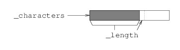
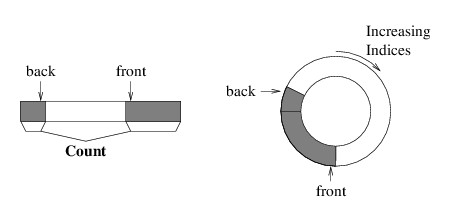
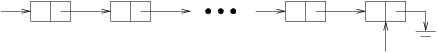
Data types in C# come in two distinct flavors: value types and reference types. In order to understand the distinction, it helps to consider how space is allocated in C#. Whenever a method is called, the space needed to execute that method is allocated from a data structure known as the call stack. The space for a method includes its local variables, including its parameters (except for out or ref parameters ). The organization of the call stack is shown in the following figure:

A picture of the call stack should appear here A picture of the call stack should appear here

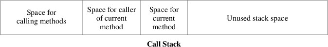
When the currently-running method makes a method call, space for that method is taken from the beginning of the unused stack space. When the currently-running method returns, its space is returned to the unused space. Thus, the call stack works like the array-based implementation of a stack 
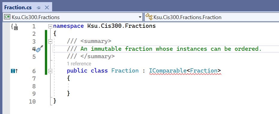
, and this storage allocation is quite efficient.

What is stored in the space allocated for a variable depends on whether the variable is for a value type or a reference type. For a value type, the value of the variable is stored directly in the space allocated for it. There are two kinds of value types: structures and enumerations . Examples of structures include numeric types such as int, double, and char. An example of an enumeration is DialogResult (see "MessageBoxes" and “File Dialogs” ).

Because value types are stored directly in variables, whenever a value is assigned to a variable of a value type, the entire value must be written to the variable. For performance reasons, value types therefore should be fairly small.

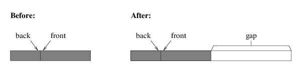
For reference types, the values are not stored directly into the space allocated for the variable. Instead, the variable stores a reference, which is like an address where the value of the variable can actually be found. When a reference type is constructed with a new expression, space for that instance is allocated from a large data structure called the heap (which is unrelated to a heap used to implement a priority queue ). Essentially, the heap is a large pool of available memory from which space of different sizes may be allocated at any time. We will not go into detail about how the heap is implemented, but suffice it to say that it is more complicated and less efficient than the stack. When space for a reference type is allocated from the heap, a reference to that space is stored in the variable. Larger data types are more efficiently implemented as reference types because an assignment to a variable of a reference type only needs to write a reference, not the entire data value.

There are three kinds of reference types: classes, interfaces , records , and delegates . Records and delegates are beyond the scope of this course.

Variables of a reference type do not need to refer to any data value. In this case, they store a value of null (variables of a value type cannot store null). Any attempt to access a method, property, or other member of a null or to apply an index to it will result in a NullReferenceException.

The fields of classes or structures are stored in a similar way, depending on whether the field is a value type or a reference type. If it is a value type, the value is stored directly in the field, regardless of whether that field belongs to an object allocated from the stack or the heap. If it is a reference type, it stores either null or a reference to an object allocated from the heap.

The difference between value types and reference types can be illustrated with the following code example:

private int[] DoSomething(int i, int j)
{
    Point a = new(i, j);
    Point b = a;
    a.X = i + j;
    int[] c = new int[10];
    int[] d = c;
    c[0] = b.X;
    return d;
}

Suppose this method is called as follows:

    int[] values = DoSomething(1, 2);

The method contains six local variables: i, j, a, b, c, and d. int is a structure, and hence a value type. Point is a structure (and hence a value type) containing public int properties X and Y, each of which can be read or modified. int[ ], however, is a reference type. Space for all six of these variables is allocated from the stack, and the space for the two Points includes space to store two int fields for each. The values 1 and 2 passed for i and j, respectively, are stored directly in these variables.

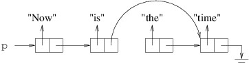
The constructor in the first line of the method above sets the X property of a to 1 and the Y property of a to 2. The next statement simply copies the value of a - i.e., the point (1, 2) - to b. Thus, when the X property of a is then changed to 3, b is unchanged - it still contains the point (1, 2).

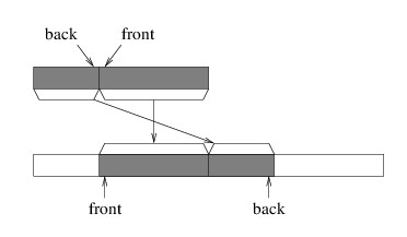
On the other hand, consider what happens when something similar is done with array variables. When c is constructed, it is assigned a new array allocated from the heap and containing 10 locations. These 10 locations are automatically initialized to 0. However, because an array is a reference type, the variable c contains a reference to the actual array object, not the array itself. Thus, when c is copied to d, the array itself is not copied - the reference to the array is copied. Consequently, d and c now refer to the same array object, not two different arrays that look the same. Hence, after we assign c[0] a value of 1, d[0] will also contain a value of 1 because c and d refer to the same array object. (If we want c and d to refer to different array objects, we need to construct a new array for each variable and make sure each location of each array contains the value we want.) The array returned therefore resides on the heap, and contains 1 at index 0, and 0 at each of its other nine locations. The six local variables are returned to unused stack space; however, because the array was allocated from the heap, the calling code may continue to use it.

It is sometimes convenient to be able to store a null in a variable of a value type. For example, we may want to indicate that an int variable contains no meaningful value. In some cases, we can reserve a specific int value for this purpose, but in other cases, there may be no int value that does not have some other meaning within the context. In such cases, we can use the ? operator to define a nullable version of a value type; e.g.,

int? i = null;

We can do this with any value type. Nullable value types such as int? are the only value types that can store null.

Beginning with C# version 8.0, similar annotations using the ? operator are allowed for reference types. In contrast to its use with value types, this operator has no effect on the code execution when it is used with a reference type. Instead, such annotations are used to help programmers to avoid NullReferenceExceptions. For example, the type string is used for variables that should never be null, but string? is used for variables that might be null. Assigning null to a string variable will not throw an exception (though it might lead to a NullReferenceException later); however, starting with .NET 6, the compiler will generate a warning whenever it cannot determine that a value assigned to a non-nullable variable is not null. One way to avoid this warning is to use the nullable version of the type; e.g.,

string? s = null;

The compiler uses a technique called static analysis to try to determine whether a value assigned to a variable of a non-nullable reference type is non-null. This technique is limited, resulting in many cases in which the value assigned cannot be null, but the compiler gives a warning anyway. (This technique is especially limited in its ability to analyze arrays.) In such cases, the null-forgiving operator ! can be used to remove the warning. Whenever you use this operator, the CIS 300 style requirements specify that you must include a comment explaining why the value assigned cannot be null (see “Comments” ).

For example, a StreamReader ’s ReadLine method returns null when there are no more lines left in the stream, but otherwise returns a non-null string (see “Advanced Text File I/O” ). We can use the StreamReader’s EndOfStream property to determine whether all lines have been read; for example, if input is a StreamReader:

while (!input.EndOfStream)
{
    string line = input.ReadLine();
    
    // Process the line
}

However, because ReadLine has a return type of string? and the type of line is string, the compiler generates a warning - even though ReadLine will never return null in this context. We can eliminate the warning as follows:

while (!input.EndOfStream)
{
    // Because input is not at the end of the stream, ReadLine won't return null.
    string line = input.ReadLine()!;
    
    // Process the line
}

Because classes are reference types, it is possible for the definition of a class C to contain one or more fields of type C or, more typically, type C?; for example:

public class C
{
    private C? _nextC;
    . . .
}

Such circularity would be impossible for a value type because there would not be room for anything else if we tried to include a value of type C? within a value of type C. However, because C is a class, and hence a reference type, _nextC simply contains either null or a reference to some object of type C. When the runtime system constructs an instance of type C, it just needs to make it large enough to hold a reference, along with any other fields defined within C. Such recursive definitions are a powerful way to link together many instances of a type. See “Linked Lists ” and “Trees ” for more information.

Because all types in C# are subtypes of object, which is a reference type, every value type is a subtype of at least one reference type (however, value types cannot themselves have subtypes). It is therefore possible to assign an instance of a value type to a variable of a reference type; for example:

object x = 3;

When this is done, a boxed version of the value type is constructed, and the value copied to it. The boxed version of the value type is just like the original value type, except that it is allocated from the heap and accessed by reference, not by value. A reference to this boxed version is then assigned to the variable of the reference type. Note that multiple variables of the reference type may refer to the same boxed instance of the value type. Note also that boxing may also occur when passing parameters. For example, suppose we have a method:

private object F(object x)
{

}

If we call F with a parameter of 3, then 3 will need to be copied to a boxed int, and a reference to this boxed int will be assigned to x within F.

Enumerations

An enumeration is a value type containing a set of named constants. An example of an enumeration is DialogResult (see "MessageBoxes" and “File Dialogs” ). The DialogResult type contains the following members:

  • DialogResult.Abort
  • DialogResult.Cancel
  • DialogResult.Ignore
  • DialogResult.No
  • DialogResult.None
  • DialogResult.OK
  • DialogResult.Retry
  • DialogResult.Yes

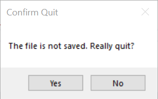
Each of the above members has a different constant value. In many cases, we are not interested in the specific value of a given member. Instead, we are often only interested in whether two expressions of this type have the same value. For example, the following code fragment is given in the "MessageBoxes" section:

DialogResult result = MessageBox.Show("The file is not saved. Really quit?", "Confirm Quit", MessageBoxButtons.YesNo);
if (result == DialogResult.Yes)
{
    Application.Exit();
}

In the if-statement above, we are only interested in whether the user closed the MessageBox with the “Yes” button; i.e., we want to know whether the Show method returned the same value as DialogResult.Yes. For this purpose, we don’t need to know anything about the value of DialogResult.Yes or any of the other DialogResult members.

However, there are times when it is useful to know that the values in an enumeration are always integers. Using a cast , we can assign a member of an enumeration to an int variable or otherwise use it as we would an int; for example, after the code fragment above, we can write:

int i = (int)result;

As a more involved example, we can loop through the values of an enumeration:

for (DialogResult r = 0; (int)r < 8; r++)
{
    MessageBox.Show(r.ToString());
}

The above loop will display 8 MessageBoxes in sequence, each displaying the name of a member of the enumeration (i.e., “None”, “OK”, etc.).

Variables of an enumeration type may be assigned any value of the enumeration’s underlying type (usually int, as we will discuss below). For example, if we had used the condition (int)r < 10 in the above for statement, the loop would continue two more iterations, showing 8 and 9 in the last two MessageBoxes.

An enumeration is defined using an enum statement, which is similar to a class statement except that in the simplest case, the body of an enum is simply a listing of the members of the enumeration. For example, the DialogResult enumeration is defined as follows:

public enum DialogResult
{
    None, OK, Cancel, Abort, Retry, Ignore, Yes, No
}

This definition defines DialogResult.None as having the value 0, DialogResult.OK as having the value 1, etc.

As mentioned above, each enumeration has underlying type. By default, this type is int, but an enum statement may specify another underlying type, as follows:

public enum Beatles : byte
{
    John, Paul, George, Ringo
}

The above construct defines the underlying type for the enumeration Beatles to be byte; thus, a variable of type Beatles may be assigned any byte value. The following integer types may be used as underlying types for enumerations:

  • byte (0 through 255)
  • sbyte (-128 through 127)
  • short (-32,768 through 32,767)
  • ushort (0 through 65,535)
  • int (-2,147,483,648 through 2,147,483,647)
  • uint (0 through 4,294,967,295)
  • long (-9,223,372,036,854,775,808 through 9,223,372,036,854,775,807)
  • ulong (0 through 18,446,744,073,709,551,615)

It is also possible to define members of an enumeration so that they are not simply the values 0, 1, etc. For example, we might alter the Beatles enumeration as follows:

public enum Beatles : byte
{
    John = 1, Paul, George = 5, Ringo
}

This defines the following values for the members:

  • Beatles.John: 1
  • Beatles.Paul: 2
  • Beatles.George: 5
  • Beatles.Ringo: 6

Thus, if a value is explicitly assigned to a member, that member takes on that value; otherwise, that member takes on the next value greater than the previous member listed, or 0 if that member is the first listed. Note that using this technique, it is possible to define two members with the same value, although this is usually undesirable. If assigning values in this way would lead to a value outside the range of the underlying type, a syntax error results (for example, if George were assigned 255 in the above definition, thus causing Ringo to have a value outside the range of a byte).

One reason we might want to define explicit values for members of an enumeration is if we want to use the members as flags. For example, one of the MessageBox.Show methods takes as one of its parameters a MessageBoxOptions , which is an enumeration containing the following members:

  • MessageBoxOptions.DefaultDesktopOnly
  • MessageBoxOptions.RightAlign
  • MessageBoxOptions.RtlReading
  • MessageBoxOptions.ServiceNotification

The meaning of each of these members is unimportant for the purposes of this discussion. The point is that the values of these members are chosen in such a way that more than one of them can be combined into a single value. The way this is done is to define each member as a different power of 2. The binary representation of a power of 2 contains exactly one bit with a value of 1. Thus, these values can be combined using a logical OR operator, and the original values can be retrieved using a logical AND operator.

For example, suppose the MessageBoxOptions enumeration is defined as follows:

public enum MessageBoxOptions
{
    DefaultDesktopOnly = 1,
    RightAlign = 2,
    RtlReading = 4,
    ServiceNotification = 8
}
Note

The definition in .NET 6 uses different powers of 2, but the priciple is the same.

Now suppose we want to create a MessageBox that will be displayed on the default desktop with right-aligned text. We can combine these options using the expression

MessageBoxOptions.DefaultDesktopOnly | MessageBoxOptions.RightAlign

This expression combines corresponding bits of the two operands using a logical OR. Recall that the logical OR of two bits is 1 if at least one of the two bits is 1. If both operands are 0, the result is 0. In this example, the operands have a 1 in different bit locations. When we combine them using logical OR, both of these bit positions will contain a 1:

0000 0000 0000 0000 0000 0000 0000 0001
0000 0000 0000 0000 0000 0000 0000 0010
---------------------------------------
0000 0000 0000 0000 0000 0000 0000 0011

We can therefore specify both of these options to the Show method as folows:

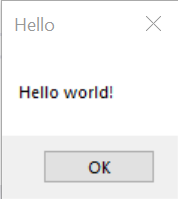
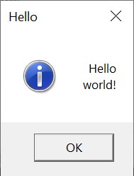
MessageBox.Show("Hello\nworld!", "Hello", MessageBoxButtons.OK,
    MessageBoxIcon.Information, MessageBoxDefaultButton.Button1, 
    MessageBoxOptions.DefaultDesktopOnly |
    MessageBoxOptions.RightAlign);

The \n in the above example specifies the end of a line; hence, “Hello” and “world!” will be displayed on separate lines, aligned on the right:

A picture of a dialog should appear here.

The Show method determines which bits are 1 in the MessageBoxOptions parameter using a logical AND. Recall that a logical AND of two bits is 1 only if both bits are 1. In all othercases, the result is 0. Suppose, then, that options is a MessageBoxOptions variable with an unknown value. Because each named member of the MessageBoxOptions enumeration (e.g., MessageBoxOptions.RightAlign) has exactly one bit with a value of 1, an expression like

options & MessageBoxOptions.RightAlign

can have only two possible values:

  • If the bit position containing the 1 in MessageBoxOptions.RightAlign also contains a 1 in options, then the expression’s value is MessageBoxOptions.RightAlign.
  • Otherwise, the expression’s value is 0.

Thus, the Show method can use code like:

if ((options & MessageBoxOptions.RightAlign) == MessageBoxOptions.RightAlign)
{
    // Code to right-align the text
}
else
{
    // Code to left-align the text
}

Defining enumerations to be used as flags in this way can be made easier by writing the powers of 2 in hexadecimal, or base 16. Each hex digit contains one of 16 possible values: the ten digits 0-9 or the six letters a-f (in either lower or upper case). A hex digit is exactly four bits; hence, the hex values containing one occurrence of either 1, 2, 4, or 8, with all other digits 0, are exactly the powers of 2. To write a number in hex in a C# program, start with 0x, then give the hex digits. For example, we can define the following enumeration to represent the positions a baseball player is capable of playing:

public enum Positions
{
    Pitcher = 0x1,
    Catcher = 0x2,
    FirstBase = 0x4,
    SecondBase = 0x8,
    ThirdBase = 0x10,
    Shortstop = 0x20,
    LeftField = 0x40,
    CenterField = 0x80,
    RightField = 0x100
}

We can then encode that a player is capable of playing 1st base, left field, center field, or right field with the expression:

Positions.FirstBase | Positions.LeftField | Positions.CenterField | Positions.RightField

This expression would give a value having four bit positions containing 1:

0000 0000 0000 0000 0000 0001 1100 0100

For more information on enumerations, see the section, Enumeration Types in the C# Reference.

Structures

A structure is similar to a class, except that it is a value type , whereas a class is a reference type . A structure definition looks a lot like a class definition; for example, the following defines a structure for storing information associated with a name:

/// <summary>
/// Stores a frequency and a rank.
/// </summary>
public readonly struct FrequencyAndRank
{
    /// <summary>
    /// Gets the Frequency.
    /// </summary>
    public float Frequency { get; }

    /// <summary>
    /// Gets the Rank.
    /// </summary>
    public int Rank { get; }

    /// <summary>
    /// Initializes a FrequencyAndRank with the given values.
    /// </summary>
    /// <param name="freq">The frequency.</param>
    /// <param name="rank">The rank.</param>
    public FrequencyAndRank(float freq, int rank)
    {
        Frequency = freq;
        Rank = rank;
    }

    /// <summary>
    /// Obtains a string representation of the frequency and rank.
    /// </summary>
    /// <returns>The string representation.</returns>
    public override string ToString()
    {
        return Frequency + ", " + Rank;
    }
}

Note that the above definition looks just like a class definition, except that the keyword struct is used instead of the keyword class, and the readonly modifier is used. The readonly modifier cannot be used with a class definition, but is often used with a structure definition to indicate that the structure is immutable. The compiler then verifies that the structure definition does not allow any fields to be changed; for example, it verifies that no property has a set accessor.

A structure can be defined anywhere a class can be defined. However, one important restriction on a structure definition is that no field can be of the same type as the structure itself. For example, the following definition is not allowed:

public struct S
{
    private S _nextS;
}

The reason for this restriction is that because a structure is a value type, each instance would need to contain enough space for another instance of the same type, and this instance would need enough space for another instance, and so on forever. This type of circular definition is prohibited even if it is indirect; for example, the following is also illegal:

public struct S
{
    public T NextT { get; }
}

public struct T
{
    public S? NextS { get; }
}

Because the NextT property uses the default implementation, each instance of S contains a hidden field of type T. Because T is a value type, each instance of S needs enough space to store an instance of T. Likewise, because the NextS property uses the default implementation, each instance of T contains a hidden field of type S?. Because S is a value type, each instance of T - and hence each instance of S - needs enough space to store an instance of S?, which in turn needs enough space to store an instance of S. Again, this results in circularity that is impossible to satisfy.

Any structure must have a constructor that takes no parameters. If one is not explicitly provided, a default constructor containing no statements is included. If one is explicitly provided, it must be public. Thus, an instance of a structure can always be constructed using a no-parameter constructor. If no code for such a constructor is provided, each field that does not contain an initializer is set to its default value.

If a variable of a structure type is assigned its default value , each of its fields is set to its default value, regardless of any initializers in the structure definition. For example, if FrequencyAndRank is defined as above, then the following statement will set both x.Frequency and x.Rank to 0:

FrequencyAndRank x = default;
Warning

Because the default value of a type can always be assigned to a variable of that type, care should be taken when including fields of reference types within a structure definition. Because the default instance of this structure will contain null values for all fields of reference types, these fields should be defined to be nullable . The compiler provides no warnings about this.

For more information on structures, see the section, “Structure types” in the C# Language Reference.

The decimal Type

A decimal is a structure representing a floating-point decimal number. The main difference between a decimal and a float or a double is that a decimal can store any value that can be written using no more than 28 decimal digits, a decimal point, and optionally a ‘-’, without rounding. For example, the value 0.1 cannot be stored exactly in either a float or a double because its binary representation is infinite (0.000110011…); however, it can be stored exactly in a decimal. Various types, such as int, double, or string, may be converted to a decimal using a Convert.ToDecimal method; for example, if i is an int, we can convert it to a decimal with:

decimal d = Convert.ToDecimal(i);

A decimal is represented internally with the following three components:

  • A 96-bit value v storing the digits (0 ≤ v ≤ 79,228,162,514,264,337,593,543,950,335).
  • A sign bit s, where 1 denotes a negative value.
  • A scale factor d to indicate where the decimal point is (0 ≤ d ≤ 28).

The value represented is then (-1)sv/10d. For example, 123.456 can be represented by setting v to 123,456, s to 0, and d to 3.

Read-Only and Constant Fields

Field declarations may contain one of the the keywords readonly or const to indicate that these fields will always contain the same values. Such declarations are useful for defining a value that is to be used throughout a class or structure definition, or throughout an entire program. For example, we might define:

public class ConstantsExample
{
    public readonly int VerticalPadding = 12;

    private const string _humanPlayer = "X";

    . . .

}

Subsequently throughout the above class, the identifier _humanPlayer will refer to the string, “X”. Because VerticalPadding is public, the VerticalPadding field of any instance of this ConstantsExample will contain the value 12 throughout the program. Such definitions are useful for various reasons, but perhaps the most important is that they make the program more maintainable. For example, VerticalPadding may represent some distance within a graphical layout. At some point in the lifetime of the software, it may be decided that this distance should be changed to 10 in order to give a more compact layout. Because we are using a readonly field rather than a literal 12 everywhere this distance is needed, we can make this change by simply changing the 12 in the above definition to 10.

When defining a const field, an initializer is required. The value assigned by the initializer must be a value that can be computed at compile time. For this reason, a constant field of a reference type can only be a string or null. The assigned value may be an expression, and this expression may contain other const fields, provided these definitions don’t mutually depend on each other. Thus, for example, we could add the following to the above definition:

private const string _paddedHumanPlayer = " " + _humanPlayer + " ";

const fields may not be declared as static , as they are already implicitly static.

A readonly field differs from a const field mainly in that it is initialized at runtime, whereas a const field is initialized at compile time. This difference has several ramifications. First, a readonly field may be initialized in a constructor as an alternative to using an initializer. Second, a readonly field may be either static or non-static. These differences imply that in different instances of the same class or structure, a readonly field may have different values.

One final difference between a readonly field and a const field is that a readonly field may be of any type and contain any value. Care must be taken, however, when defining a readonly reference type. For example, suppose we define the following:

private readonly string[] _names = { "Peter", "Paul", "Mary" };

Defining _names to be readonly guarantees that this field will always refer to the same array after its containing instance is constructed. However, it does not guarantee that the three array locations will always contain the same values. For this reason, the use of readonly for public fields of mutable reference types is discouraged.

readonly is preferred over const for a public field whose value may change later in the software lifecycle. If the value of a public const field is changed by a code revision, any code using that field will need to be recompiled to incorporate that change.

Properties

A property is used syntactically like a field of a class or structure, but provides greater flexibility in implementation. For example, the string class contains a public property called Length . This property is accessed in code much as if it were a public int field; i.e., if s is a string variable, we can access its Length property with the expression s.Length, which evaluates to an int. If Length were a public int field, we would access it in just the same way. However, it turns out that we cannot assign a value to this property, as we can to a public field; i.e., the statement,

s.Length = 0;

is not allowed. The reason for this limitation is that properties can be defined to restrict whether they can be read from or written to. The Length property is defined so that it can be read from, but not written to. This flexibility is one of the two main differences between a field and a property. The other main difference has to do with maintainability and is therefore easier to understand once we see how to define a property.

Suppose we wish to provide full read/write access to a double value. Rather than defining a public double field, we can define a simple double property as follows:

public double X { get; set; }

This property then functions just like a public field - the get keyword allows code to read from the property, and the set keyword allows code to write to the property. A property definition requires at least one of these keywords, but one of them may be omitted to define a read-only property (if set is omitted) or a write-only property (if get is omitted). For example, the following defines X to be a read-only property:

public double X { get; }

Although this property is read-only, the constructor for the class or structure containing this definition is allowed to initialize it. Sometimes, however we want certain methods of the containing class or structure to be able to modify the property’s value without allowing user code to do so. To accomplish this, We can define X in this way:

public double X { get; private set; }

The above examples are the simplest ways to define properties. They all rely on the default implementation of the property. Unlike a field, the name of the property is not actually a variable; instead, there is a hidden variable that is automatically defined. The only way this hidden variable can be accessed is through the property.

Warning

Don’t define a private property using the default implementation. Use a private field instead.

The distinction between a property and its hidden variable may seem artificial at first. However, the real flexibility of a property is revealed by the fact that we can define our own implementation, rather than relying on the default implementation. For example, suppose a certain data structure stores a StringBuilder called _word, and we want to provide read-only access to its length. We can facilitate this by defining the following property:

public int WordLength
{
    get => _word.Length;
}

In fact, we can abbreviate this definition as follows:

public int WordLength => _word.Length;

In this case, the get keyword is implied. In either case, the code to the right of the “=>” must be an expression whose type is the same as the property’s type. Note that when we provide such an expression, there is no longer a hidden variable, as we have provided explicit code indicating how the value of the property is to be computed.

We can also provide an explicit implementation for the set accessor. Suppose, for example, that we want to allow the user read/write access to the length of _word. In order to be able to provide write access, we must be able to acquire the value that the user wishes to assign to the length. C# provides a keyword value for this purpose - its type is the same as the type of the property, and it stores the value that user code assigns to the property. Hence, we can define the property as follows:

public int WordLength
{
    get => _word.Length;
    set => _word.Length = value;
}

It is this flexibility in defining the implementation of a property that makes public properties more maintainable than public fields. Returning to the example at the beginning of this section, suppose we had simply defined X as a public double field. As we pointed out above, such a field could be used by user code in the same way as the first definition of the property X. However, a field is part of the implementation of a class or structure. By making it public, we have exposed part of the implementation to user code. This means that if we later change this part of the implementation, we will potentially break user code that relies on it. If, instead, we were to use a property, we can then change the implementation by modifying the get and/or set accessors. As long as we don’t remove either accessor (or make it private), such a change is invisible to user code. Due to this maintainability, good programmers will never use public fields (unless they are constants ); instead, they will use public properties.

In some cases, we need more than a single to expression to define a get or set accessor. For example, suppose a data structure stores an int[ ] _elements, and we wish to provide read-only access to this array. In order to ensure read-only access, we don’t want to give user code a reference to the array, as the code would then be able to modify its contents. We therefore wish to make a copy of the array, and return that array to the user code (though a better solution might be to define an indexer ). We can accomplish this as follows:

public int[ ] Elements
{
    get
    {
        int[] temp = new int[_elements.Length];
        _elements.CopyTo(temp, 0);
        return temp;
    }
}

Thus, arbitrary code may be included within the get accessor, provided it returns a value of the appropriate type; however, it is good programming practice to avoid changing the fields of a class or structure within the get accessor of one of its properties. In a similar way, arbitrary code may be used to implement a set accessor. As we can see from this most general way of defining properties, they are really more like methods than fields.

Given how similar accessors are to methods, we might also wonder why we don’t just use methods instead of properties. In fact, we can do just that - properties don’t give any functional advantage over methods, and in fact, some object-oriented languages don’t have properties. The advantage is stylistic. Methods are meant to perform actions, whereas properties are meant to represent entities. Thus, we could define methods GetX and SetX to provide access to the private field _x; however, it is stylistically cleaner to define a property called X.

Indexers

Recall that the System.Collections.Generic.Dictionary<TKey, TValue> class (see “The Dictionary<TKey, TValue> Class” ) allows keys to be used as indices for the purpose of adding new keys and values, changing the value associated with a key, and retrieving the value associated with a key in the table. In this section, we will discuss how to implement this functionality.

An indexer in C# is defined using the following syntax:

public TValue this[TKey k]
{
    get
    {
        // Code to retrieve the value with key k
    }
    set
    {
        // Code to associate the given value with key k
    }
}

Note the resemblance of the above code to the definition of a property. The biggest differences are:

  • In place of a property name, an indexer uses the keyword this.
  • The keyword this is followed by a nonempty parameter list enclosed in square brackets.

Thus, an indexer is like a property with parameters. The parameters are the indices themselves; i.e., if d is a Dictionary<TKey, TValue> and key is a TKey, d[key] invokes the indexer with parameter key. In general, either the get accessor or the set accessor may be omitted, but at least one of them must be included. As in a property definition, the set accessor can use the keyword value for the value being assigned - in this case, the value to be associated with the given key. The value keyword and the return type of the get accessor will both be of type TValue, the type given prior to the keyword this in the above code.

We want to implement the indexer to behave in the same way as the indexer for System.Collections.Generic.Dictionary<TKey, TValue>. Thus, the get accessor is similar to the TryGetValue method, as outlined in “A Simple Hash Table Implementation” , with a few important differences. First, the get accessor has no out parameter. Instead, it returns the value that TryGetValue assigns to its out parameter when the key is found. When the key is not found, because it can’t return a bool to indicate this, it instead throws a KeyNotFoundException.

Likewise, the set accessor is similar to the Add method, as outlined in “A Simple Hash Table Implementation” . However, whereas the Add method has a TValue parameter through which to pass the value to be associated with the given key, the set accessor gets this value from the value keyword. Furthermore, we don’t want the set accessor to throw an exception if the key is found. Instead, we want it to replace the Data of the cell containing this key with a new KeyValuePair containing the key with the new value.

The Keywords static and this

Object-oriented programming languages such as C# are centered on the concept of an object. Class and structure definitions give instructions for constructing individual objects of various types, normally by using the new keyword. When an object is constructed, it has its own fields in which values may be stored. Specifically, if type T has an int field called _length, then each object of type T will have have such a field, and each of these fields may store a different int. Thus, for example, if x and y are instances of type T, then x._length may contain 7, while y._length may contain 12.

Likewise, we can think of each object as having its own methods and properties, as when any of these methods or properties use the fields of the containing class or structure, they will access the fields belonging to a specific object. For example, if type T contains an Add method that changes the value stored in the _length filed, then a call x.Add will potentially change the value stored in x._length.

However, there are times when we want to define a field, method, or property, but we don’t want it associated with any specific object. For example, suppose we want to define a unique long value for each instance of some class C. We can define a private long field _id within this class and give it a value within its constructor. But how do we get this value in a way that ensures that it is unique? One way is to define a private static long field _nextId, as in the following code:

public class C
{
    private static long _nextId = 0;

    private long _id;

    public C()
    {
        _id = _nextId;
        _nextId++;
    }

    // Other members could also be defined.
}

By defining _nextId to be static, we are specifying that each instance of C will not contain a _nextId field, but instead, there is a single _nextId field belonging to the entire class. As a result, code belonging to any instance of C can access this one field. Thus, each time an instance of C is constructed, this one field is incremented. This field therefore acts as a counter that keeps track of how many instances of C have been constructed. On the other hand, because _id is not static, each instance of C contains an _id field. Thus, when the assignment,

_id = _nextId;

is done, the value in the single _nextId field is copied to the value of the _id field belonging to the instance being constructed. Because the single _nextId field is incremented every time a new instance of C is constructed, each instance receives a different value for _id.

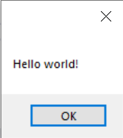
We can also define static methods or properties. For example, the MessageBox.Show(string text) method is static. Because it is static, we don’t need a MessageBox object in order to call this method - we simply call something like:

MessageBox.Show("Hello world!");

static methods can also be useful for avoiding NullReferenceExceptions. For example, there are times when we want to determine whether a variable x contains null, but x is of an unknown type (perhaps its type is defined by some type parameter T). In such a case, we cannot use == to make the comparison because == is not defined for all types. Furthermore, the following will never work:

if (x.Equals(null))
{

}

Such code will compile, but if x is null, then calling its Equals method will throw a NullReferenceException. In all other cases, the if-condition will evaluate to false. Fortunately, a static Equals method is available to handle this situation:

if (Equals(x, null))
{

}

Because this method is defined within the object class, which is a supertype of every other type in C#, we can refer to this method without specifying the containing class, just as if we had defined it in the class or structure we are writing. Because this method does not belong to individual objects, we don’t need any specific object available in order to call it. It therefore avoids a NullReferenceException.

Because a static method or property does not belong to any instance of its type, it cannot access any non-static members directly, as they all belong to specific instances of the type. If however, the code has access to a specific instance of the type (for example, this instance might be passed as a parameter), the code may reference non-static members of that instance. For example, suppose we were to add to the class C above a method such as:

public static int DoSomething(C x)
{

}

Code inside this method would be able to access _nextID, but not _id. Furthermore, it would be able to access any static methods or properties contained in the class definition, as well as all constructors, but no non-static methods or properties. However, it may access x._id, as well as any other members of x.

Code within a constructor or a non-static method or property can also access the object that contains it by using the keyword this. Thus, in the constructor code above, we could have written the line

_id = _nextId;

as

this._id = _nextId;

In fact, the way we originally wrote the code is simply an abbreviation of the above line. Another way of thinking of the restrictions on code within a static method or property is that this code cannot use this, either explicitly or implicitly.

out and ref Parameters

Normally, when a method is called, the call-by-value mechanism is used. Suppose, for example, we have a method:

private void DoSomething(int k)
{

}

We can call this method with a statement like:

DoSomething(n);

provided n is an initialized variable consistent with the int type. For example, suppose n is an int variable containing a value of 28. The call-by-value mechanism works by copying the value of n (i.e., 28) to k. Whatever the DoSomething method may do to k has no effect on n — they are different variables. The same can be said if we had instead passed a variable k — the k in the calling code is still a different variable from the k in the DoSomething method. Finally, if we call DoSomething with an expression like 9 + n, the mechanism is the same.

If a parameter is of a reference type , the same mechanism is used, but it is worth considering that case separately to see exactly what happens. Suppose, for example, that we have the following method:

private void DoSomethingElse(int[] a)
{
    a[0] = 1;
    a = new int[10];
    a[1] = 2;
}

Further suppose that we call this method with

int[] b = new int[5];
DoSomethingElse(b);

The initialization of b above assigns to b a reference to an array containing five 0s. The call to DoSomethingElse copies the value of b to a. Note, however, that the value of b is a reference; hence, after this value is copied, a and b refer to the same five-element array. Therefore, when a[0] is assigned 1, b[0] also becomes 1. When a is assigned a new array, however, this does not affect b, as b is a different variable — b still refers to the same five-element array. Furthermore, when a[1] is assigned a value of 2, because a and b now refer to different arrays, the contents of b are unchanged. Thus, when DoSomethingElse completes, b will refer to a five-element array whose element at location 0 is 1, and whose other elements are 0.

While the call-by-value mechanism is used by default, another mechanism, known as the call-by-reference mechanism, can be specified. When call-by-reference is used, the parameter passed in the calling code must be a variable, not a property or expression. Instead of copying the value of this variable into the corresponding parameter within the method, this mechanism causes the variable within the method to be an alias for the variable being passed. In other words, the two variables are simply different names for the same underlying variable (consequently, the types of the two variables must be identical). Thus, whatever changes are made to the parameter within the method are reflected in the variable passed to the method in the calling code as well.

One case in which this mechanism is useful is when we would like to have a method return more than one value. Suppose, for example, that we would like to find both the maximum and minimum values in a given int[ ]. A return statement can return only one value. Although there are ways of packaging more than one value together in one object, a cleaner way is to use two parameters that use the call-by-reference mechanism. The method can then change the values of these variables to the maximum and minimum values, and these values would be available to the calling code.

Specifically, we can define the method using out parameters:

private void MinimumAndMaximum(int[] array, out int min, out int max)
{
    min = array[0];
    max = array[0];
    for (int i = 1; i < array.Length; i++)
    {
        if (array[i] < min)
        {
            min = array[i];
        }
        if (array[i] > max)
        {
            max = array[i];
        }
    }
}

The out keyword in the first line above specifies the call-by-reference mechanism for min and max. We could then call this code as follows, assuming a is an int[ ] containing at least one element:

int minimum;
int maximum;
MinimumAndMaximum(a, out minimum, out maximum);

When this code completes, minimum will contain the minimum element in a and maximum will contain the maximum element in a.

Warning

When using out parameters, it is important that the keyword out is placed prior to the variable name in both the method call and the method definition. If you omit this keyword in one of these places, then the parameter lists won’t match, and you’ll get a syntax error to this effect.

Tip

As a shorthand, you can declare an out parameter in the parameter list of the method call. Thus, the above example could be shortened to the following single line of code:

MinimumAndMaximum(a, out int minimum, out int maximum);

Note that out parameters do not need to be initialized prior to the method call in which they are used. However, they need to be assigned a value within the method to which they are passed. Another way of using the call-by-reference mechanism places a slightly different requirement on where the variables need to be initialized. This other way is to use ref parameters. The only difference between ref parameters and out parameters is that ref parameters must be initialized prior to being passed to the method. Thus, we would typically use an out parameter when we expect the method to assign it its first value, but we would use a ref parameter when we expect the method to change a value that the variable already has (the method may, in fact, use this value prior to changing it).

For example, suppose we want to define a method to swap the contents of two int variables. We use ref parameters to accomplish this:

private void Swap(ref int i, ref int j)
{
    int temp = i;
    i = j;
    j = temp;
}

We could then call this method as follows:

int m = 10;
int n = 12;
Swap(ref m, ref n);

After this code is executed, m will contain 12 and n will contain 10.

The foreach Statement

C# provides a foreach statement that is often useful for iterating through the elements of certain data structures. A foreach can be used when all of the following conditions hold:

  1. The data structure is a subtype of either IEnumerable or IEnumerable<T> for some type T.
  2. You do not need to know the locations in the data structure of the individual elements.
  3. You do not need to modify the data structure with this loop.
Warning

Many of the data structures provided to you in CIS 300, as well as many that you are to write yourself for this class, are not subtypes of either of the types mentioned in 1 above. Consequently, we cannot use a foreach loop to iterate through any of these data structures. However, most of the data structures provided in the .NET Framework, as well as all arrays, are subtypes of one of these types.

For example, the string class is a subtype of both IEnumerable and IEnumerable<Char>. To see that this is the case, look in the documentation for the string class . In the “Implements” section, we see all of the interfaces implemented by string. Because string implements both of these interfaces, it is a subtype of each. We can therefore iterate through the elements (i.e., the characters) of a string using a foreach statement, provided we don’t need to know the location of each character in the string (because a string is immutable, we can’t change its contents).

Suppose, for example, that we want to find out how many times the letter ‘i’ occurs in a string s. Because we don’t need to know the locations of these occurrences, we can iterate through the characters with a foreach loop, as follows:

int count = 0;
foreach (char c in s)
{
    if (c == 'i')
    {
        count++;
    }
}

The foreach statement requires three pieces of information:

  • The type of the elements in the data structure (char in the above example).
  • The name of a new variable (c in the above example). The type of this variable will be the type of the elements in the data structure (i.e., char in the above example). It will take on the values of the elements as the loop iterates.
  • Following the keyword in, the data structure being traversed (s in the above example).

The loop then iterates once for each element in the data structure (unless a statement like return or break causes it to terminate prematurely). On each iteration, the variable defined in the foreach statement stores one of the elements in the data structure. Thus, in the above example, c takes the value of a different character in s on each iteration. Note, however, that we have no access to the location containing c on any particular iteration - this is why we don’t use a foreach loop when we need to know the locations of the elements. Because c takes on the value of each character in s, we are able to count how many of them equal ‘i’.

Occasionally, it may not be obvious what type to use for the foreach loop variable. In such cases, if the data structure is a subtype of IEnumerable<T>, then the type should be whatever type is used for T. Otherwise, it is safe to use object. Note, however, that if the data structure is not a subtype of IEnumerable<T>, but you know that the elements are some specific subtype of object, you can use that type for the loop variable - the type will not be checked until the code is executed. For example, ListBox is a class that implements a GUI control displaying a list of elements. The elements in the ListBox are accessed via its Items property, which gets a data structure of type ListBox.ObjectCollection . Any object can be added to this data structure, but we often just add strings. ListBox.ObjectCollection is a subtype of IEnumerable; however, it is permissible to set up a foreach loop as follows:

foreach (string s in uxList.Items)
{

}

where uxList is a ListBox variable. As long as all of the elements in uxList.Items are strings, no exception will be thrown.

While the foreach statement provides a clean way to iterate through a data structure, it is important to keep in mind its limitations. First, it can’t even be used on data structures that aren’t subtypes of IEnumerable or IEnumerable<T>. Second, there are many cases, especially when iterating through arrays, where the processing we need to do on the elements depends on the locations of the elements. For example, consider the problem of determining whether two arrays contain the same elements in the same order. For each element of one array, we need to know if the element at the same location in the other array is the same. Because the locations are important, a foreach loop isn’t appropriate - we should use a for loop instead. Finally, a foreach should never be used to modify a data structure, as this causes unpredictable results.

Even when a foreach would work, it is not always the best choice. For example, in order to determine whether a data structure contains a given element, we could iterate through the structure with a foreach loop and compare each element to the given element. While this would work, most data structures provide methods for determining whether they contain a given element. These methods are often far more efficient than using a foreach loop.

Enumerators

As we saw in the previous section , in order for a data structure to support a foreach loop, it must be a subtype of either IEnumerable or IEnumerable<T> , where T is the type of the elements in the data structure. Thus, because Dictionary<TKey, TValue> is a subtype of IEnumerable<KeyValuePair<TKey, TValue>>, we can use a foreach loop to iterate through the key-value pairs that it stores. Likewise, because its Keys and Values properties get objects that are subtypes of IEnumerable<TKey> and IEnumerable<TValue>, respectively, foreach loops may be used to iterate through these objects as well, in order to process all the keys or all the values stored in the dictionary. IEnumerable and IEnumerable<T> are interfaces ; hence, we must define any subtypes so that they implement these interfaces. In this section, we will show how to implement the IEnumerable<T> interface to support a foreach loop.

The IEnumerable<T> interface requires two methods:

  • public IEnumerator<T> GetEnumerator()
  • IEnumerator IEnumerable.GetEnumerator()

The latter method is required only because IEnumerable<T> is a subtype of IEnumerable, and that interface requires a GetEnumerator method that returns a non-generic IEnumerator. Both of these methods should return the same object; hence, because IEnumerator<T> is also a subtype of IEnumerator, this method can simply call the first method:

IEnumerator IEnumerable.GetEnumerator()
{
    return GetEnumerator();
}

The public GetEnumerator method returns an IEnumerator<T>. In order to get instances of this interface, we could define a class that implements it; however, C# provides a simpler way to define a subtype of this interface, or, when needed, the IEnumerable<T> interface.

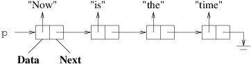
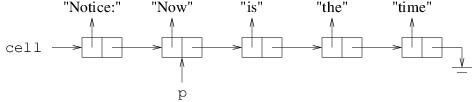
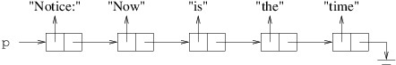
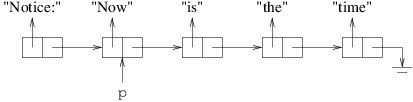
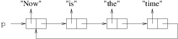
Defining such an enumerator is as simple as writing code to iterate through the elements of the data structure. As each element is reached, it is enumerated via a yield return statement. For example, suppose a dictionary implementation uses a List<KeyValuePair<TKey, TValue>> called _elements to store its key-value pairs. We can then define its GetEnumerator method as follows:

public IEnumerator<KeyValuePair<TKey, TValue>> GetEnumerator()
{
    foreach (KeyValuePair<TKey, TValue> p in _elements)
    {
        yield return p;
    }
}

Suppose user code contains a Dictionary<string, int> called d and a foreach loop structured as follows:

foreach (KeyValuePair<string, int> x in d)
{

}

Then the GetEnumerator method is executed until the yield return is reached. The state of this method is then saved, and the value p is used as the value for x in the first iteration of the foreach in the user code. When this loop reaches its second iteration, the GetEnumerator method resumes its execution until it reaches the yield return a second time, and again, the current value of p is used as the value of x in the second iteration of the loop in user code. This continues until the GetEnumerator method finishes; at this point, the loop in user code terminates.

Before continuing, we should mention that there is a simpler way of implementing the public GetEnumerator method in the above example. Because List<T> implements IEnumerable<T>, we can simply use its enumerator:

public IEnumerator> GetEnumerator()
{
    return _elements.GetEnumerator();
}

However, the first solution illustrates a more general technique that can be used when we don’t have the desired enumerator already available. For instance, continuing the above example, suppose we wish to define a Keys property to get an IEnumerable<TKey> that iterates through the keys in the dictionary. Because the dictionary now supports a foreach loop, we can define this code to iterate through the key-value pairs in the dictionary, rather than the key-value pairs stored in the List<KeyVauePair<TKey, TValue>>:

public IEnumerable<TKey> Keys
{
    get
    {
        foreach (KeyValuePair<TKey, TValue> p in this)
        {
            yield return p.Key;
        }
    }
}

The above code is more maintainable than iterating through the List<KeyValuePair<TKey, TValue>> as it doesn’t depend on the specific implementation of the dictionary.

While this technique usually works best with iterative code, it can also be used with recursion, although the translation usually ends up being less direct and less efficient. Suppose, for example, our dictionary were implemented as in “Binary Search Trees” , where a binary search tree is used. The idea is to adapt the inorder traversal algorithm. However, we can’t use this directly to implement a recursive version of the GetEnumerator method because this method does not take any parameters; hence, we can’t apply it to arbitrary subtrees. Instead, we need a separate recursive method that takes a BinaryTreeNode<KeyValuePair<TKey, TValue>> as its parameter and returns the enumerator we need. Another problem, though, is that the recursive calls will no longer do the processing that needs to be done on the children - they will simply return enumerators. We therefore need to iterate through each of these enumerators to include their elements in the enumerator we are returning:

private static IEnumerable<KeyValuePair<TKey, TValue>>
    GetEnumerable(BinaryTreeNode<KeyValuePair<TKey, TValue>>? t)
{
    if (t != null)
    {
        foreach (KeyValuePair<TKey, TValue> p in GetEnumerable(t.LeftChild))
        {
            yield return p;
        }
        yield return t.Data;
        foreach (KeyValuePair<TKey, TValue> p in GetEnumerable(t.RightChild))
        {
            yield return p;
        }
    }
}

Note that we’ve made the return type of this method IEnumerable<KeyValuePair<TKey, TValue>> because we need to use a foreach loop on the result of the recursive calls. Then because any instance of this type must have a GetEnumerator method, we can implement the GetEnumerator method for the dictionary as follows:

public IEnumerator<KeyValuePair<TKey, TValue>> GetEnumerator()
{
    return GetEnumerable(_elements).GetEnumerator();
}

In transforming the inorder traversal into the above code, we have introduced some extra loops. These loops lead to less efficient code. Specifically, if the binary search tree is an AVL tree or other balanced binary tree, the time to iterate through this enumerator is in $ O(n \lg n) $, where $ n $ is the number of nodes in the tree. The inorder traversal, by contrast, runs in $ O(n) $ time. In order to achieve this running time with an enumerator, we need to translate the inorder traversal to iterative code using a stack. However, this code isn’t easy to understand:

public IEnumerator<KeyValuePair<TKey, TValue>> GetEnumerator()
{
    Stack<BinaryTreeNode<KeyValuePair<TKey, TValue>>> s = new();
    BinaryTreeNode<KeyValuePair<TKey, TValue>>? t = _elements;
    while (t != null || s.Count > 0)
    {
        while (t != null)
        {
            s.Push(t);
            t = t.LeftChild;
        }
        t = s.Pop();
        yield return t.Data;
        t = t.RightChild;
    }
}

The switch Statement

The switch statement provides an alternative to the if statement for certain contexts. It is used when different cases must be handled based on the value of an expression that can have only a few possible results.

For example, suppose we want to display a MessageBox containing “Abort”, “Retry”, and “Ignore” buttons. The user can respond in only three ways, and we need different code in each case. Assuming message and caption are strings, we can use the following code:

switch (MessageBox.Show(message, caption, MessageBoxButtons.AbortRetryIgnore))
{
    case DialogResult.Abort:
        // Code for the "Abort" button
        break;
    case DialogResult.Retry:
        // Code for the "Retry" button
        break;
    case DialogResult.Ignore:
        // Code for the "Ignore" button
        break;
}

The expression to determine the case (in this example, the call to MessageBox.Show) is placed within the parentheses following the keyword switch. Because the value returned by this method is of the enumeration type DialogResult , it will be one of a small set of values; in fact, given the buttons placed on the MessageBox, this value must be one of three possibilities. These three possible results are listed in three case labels. Each of these case labels must begin with the keyword case, followed by a constant expression (i.e., one that can be fully evaluated by the compiler, as explained in the section, “Constant Fields” ), followed by a colon (:). When the expression in the switch statement is evaluated, control jumps to the code following the case label containing the resulting value. For example, if the result of the call to MessageBox.Show is DialogResult.Retry, control jumps to the code following the second case label. If there is no case label containing the value of the expression, control jumps to the code following the switch statement. The code following each case label must be terminated by a statement like break or return, which causes control to jump elsewhere. (This arcane syntax is a holdover from C, except that C allows control to continue into the next case.) A break statement within a switch statement causes control to jump to the code following the switch statement.

The last case in a switch statement may optionally have the case label:

default:

This case label is analogous to an else on an if statement in that if the value of the switch expression is not found, control will jump to the code following the default case label. While this case is not required in a switch statement, there are many instances when it is useful to include one, even if you can explicitly enumerate all of the cases you expect. For example, if each case ends by returning a value, but no default case is included, the compiler will detect that not all paths return a value, as any case that is not enumerated will cause control to jump past the entire switch statement. There are various ways of avoid this problem:

  • Make the last case you are handling the default case.
  • Add a default case that explicitly throws an exception to handle any cases that you don’t expect.
  • Add either a return or a throw following the switch statement (the first two options are preferable to this one).

It is legal to have more than one case label on the same code block. For example, if i is an int variable, we can use the following code:

switch (i)
{
    case 1:
        // Code for i = 1
        break;
    case 2:
    case 3:
    case 5:
    case 7:
        // Code for i = 2, 3, 5, or 7
        break;
    case 4:
    case 6:
    case 8:
        // Code for i = 4, 6, or 8
        break;
    default:
        // Code for all other values of i
        break;
}

If the value of the switch expression matches any one of the case labels on a block, control jumps to that block. The same case label may not appear more than once.

The Remainder Operator

The remainder operator % computes the remainder that results when one number is divided by another. Specifically, suppose m and n are of some numeric type, where n ≠ 0. We can then define a quotient q and a remainder r as the unique values such that:

  • qn + r = m;
  • q is an integer;
  • |qn| ≤ |m|; and
  • |r| < |n|.

Then m % n gives r, and we can compute q by:

(m - r) / n

Another way to think about m % n is through the following algorithm to compute it:

  1. Compute |m| / |n|, and remove any fractional part.
  2. If m and n have the same sign, let q be the above result; otherwise, let q be the negative of the above result.
  3. m % n is m - qn.

Examples:

  • 7 % 3 = 1
  • -9 % 5 = -4
  • 8 % -3 = 2
  • -10 % -4 = -2
  • 6.4 % 1.3 = 1.2

Visual Studio

This chapter will guide you through the use of Visual Studio 2022 and GitHub to obtain start code for your assignments, build, test, and debug graphical applications and class libraries, and submit assignment solutions. No attempt is meant to be exhaustive, as many of the features of Visual Studio are beyond the scope of CIS 300.

Note

This guide is based on Visual Studio Community 2022, version 17.6.1, released May 22, 2023. The user interface may have some differences in other versions.

Subsections of Visual Studio

Installing Visual Studio

Visual Studio Community 2022 is available on the machines we use for CIS 300 labs, as well as on machines in other lab classrooms. Students can also access Visual Studio via a remote desktop server — see the CS Department Support Wiki for details. This edition of Visual Studio is also freely available for installation on your own PC for your personal and classroom use. This section provides instructions for obtaining this software from Microsoft and installing it on your PC.

While Microsoft also produces a version of Visual Studio for Mac, we recommend the Windows version. If you don’t have a Microsoft operating system, you can obtain one for free from the Azure Portal — see the CS Department Support Wiki for details. You will need to install the operating system either on a separate bootable partition or using an emulator such as VMware Fusion. VMware Fusion is also available for free through the VMware Academic Program — see the CS Department Support Wiki for details.

To download Visual Studio Community 2022, go to Microsoft’s Visual Studio Site , and from the “Download Visual Studio” dropdown, select “Community 2022”. This should normally begin downloading an installation file; if not, click the “click here to retry” link near the top of the page. When the download has completed, run the file you downloaded. This will start the installation process.

As the installation is beginning, you will be shown a window asking for the components to be installed. Click the “Workloads” tab in this window, and select “.NET desktop development” (under “Desktop & Mobile”). You can select other workloads or components if you wish, but this workload will install all you need for CIS 300.

The first time you run Visual Studio, you will be asked to sign in to your Microsoft account. You can either do this or skip it by clicking, “Not now, maybe later.” You will then be shown a window resembling the following:

A picture of a configuration window should appear
here

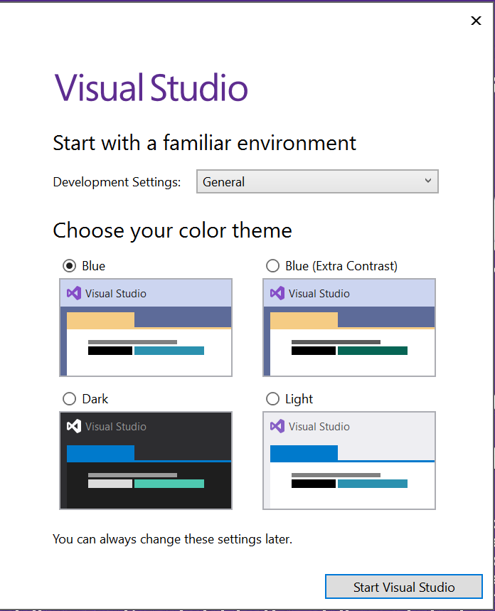
Next to “Development Settings:”, select “Visual C#”. You can select whichever color scheme you prefer. At this point, Visual Studio should be fully installed and ready to use.

Git Repositories

In CIS 300, start code for each assignment will be distributed via a Git repository. Git is a source control system integrated into Visual Studio 2022. Source control systems are powerful mechanisms for teams of programmers and other collaborators to manage multiple copies of various source files and other documents that all collaborators may be modifying. While CIS 300 does not involve teamwork, source control provides a convenient mechanism for distribution of code and submission of assignment solutions. In addition, as we will discuss later, source control provides mechanisms for accessing your code on multiple machines and for “checkpointing” your code .

At the heart of Git is the concept of a Git repository. A Git repository is essentially a folder on your local machine. As you make changes within this folder, Git tracks these changes. From time to time, you will commit these changes. If you see that you have gone down a wrong path, you can revert to an earlier commit. Git repositories may be hosted on a server such as GitHub. Various users may have copies of a Git repository on their own local machines. Git provides tools for synchronizing local repositories with the repository hosted on the server in a consistent way.

Note

The above description is a bit of an oversimplification, as the folder comprising a local copy of a repository typically contains some files and/or folders that are not part of the repository. One example of such “extra” files might be executables that are generated whenever source code within the repository is compiled. However, when Visual Studio is managing a Git repository, it does a good job of including within the repository any files the user places within the folder comprising the repository.

For each lab and homework assignment in CIS 300, you will be provided a URL that will create your own private Git repository on GitHub. The only people who will have access to your GitHub repositories are you, the CIS 300 instructors, and the CIS 300 lab assistants. These repositories will initially contain start code and perhaps data files for the respective assignments. You will copy the repository to your local machine by cloning it. When you are finished with the assignment, you will push the repository back to GitHub and submit its URL for grading. In what follows, we will explain how to create and clone a GitHub repository. Later in this chapter, we will explain how to commit changes, push a repository, and use some of the other features of Git.

Before you can access GitHub, you will need a GitHub account. If you don’t already have one, you can sign up for one at github.com . At some point after you have completed the sign-up process, GitHub will send you an email asking you to verify the email address you provided during the sign-up process. After you have done this, you will be able to set up GitHub repositories.

For each assignment in CIS 300, you will be given an invitation URL, such as:

Over the next few sections, we will be working through a simple example based on the above invitation link. If you wish to work through this example, click on the above link. You may be asked to sign in to GitHub, but once you are signed in, you will be shown a page asking you to accept the assignment. Clicking the “Accept this assignment” button will create a GitHub repository for you. You will be given a link that will take you to that repository. From that page you will be able to view all of the files in the repository.

In order to be able to use this repository, you will need to clone it to your local machine. To do this, first open Visual Studio 2022, and click on the “Clone a Repository” button on the right. In your web browser, navigate to the GitHub repository that you wish to clone, and click on the “Code” button. This will display a URL - click on the button to its right to copy this URL to your clipboard. Then go back to Visual Studio and paste this URL into the text box labeled, “Repository location”. In the text box below that, fill in a new folder you want to use for this repository on your machine, then click the “Clone” button (if you are asked to sign in to GitHub, click the link to sign in through your web browser). This will copy the Git repository from GitHub into the folder you selected, and open the solution it contains.

The following sections give an overview of how to use Visual Studio to edit and debug an application, as well as how to use Git within Visual Studio to maintain the local Git repository and synchronize it with the GitHub repository.

Visual Studio Solutions

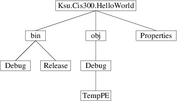
All code developed within Visual Studio 2022 must belong to one or more solutions. When you are using Visual Studio to develop a program, you will be working with a single solution. A solution will contain one or more projects. Each of these projects may belong to more than one solution. Each project typically contains several files, including source code files. Each file will typically belong to only one project. The following figure illustrates some of the possible relationships between solutions, projects, and files.

Relationships between solutions, projects, and files Relationships between solutions, projects, and files

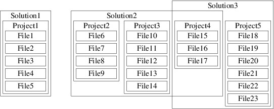
Note that in the above figure, Project4 is contained in both Solution2 and Solution3. In this section, we will focus on solutions that contain exactly one project, which in turn belongs to no other solutions (e.g., Solution1 in the above figure).

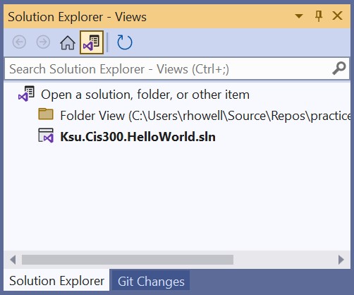
Whenever you open a solution in Studio 2022, the Solution Explorer (which you can always find on the “View” menu) will give you a view of the structure of your solution; for example, opening the solution in the repository given in the previous section may result in the following being shown in the Solution Explorer:

A picture of a Solution Explorer should appear here

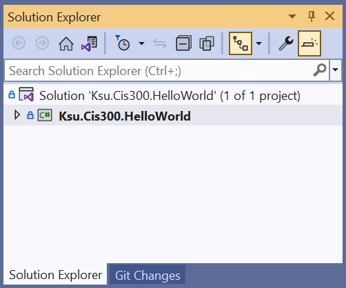
If you see the above, you will need to change to the Solution view, which you can get by double clicking the line that ends in “.sln”. This will give you the following view:

A picture of a Solution Explorer should appear
here

Warning

You ordinarily will not want to use Folder view, as this will cause files to be edited without any syntax or consistency checking. As a result, you can end up with a solution that is unusable. If your Solution Explorer ever looks like this:

A picture of a Solution Explorer in folder view should appear here

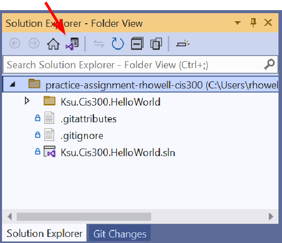
(note the indication “Folder View” at the top and the absence of any boldface line), then it is in Folder view. To return to Solution view, click the icon indicated by the arrow in the above figure. This will return the Solution Explorer to the initial view shown above, where you can double-click the solution to select Solution view.

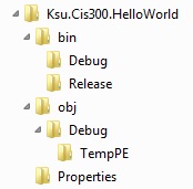
If you click on the small triangle to the left of “Ksu.Cis300.HelloWorld”, you will get a more-detailed view:

A picture of a Solution Explorer should appear here

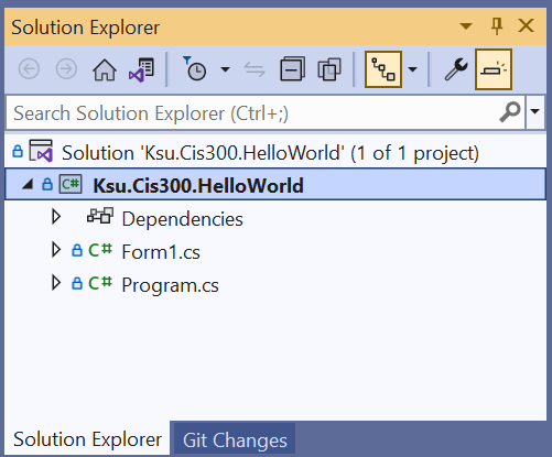
Near the top, just under the search box, is the name of the solution with an indication of how many projects it contains. Listed under the name of the solution is each project, together with the various components of the project. One of the projects is always shown in bold face. The bold face indicates that this project is the startup project; i.e., it is the project that the debugger will attempt to execute whenever it is invoked (for more details, see the section, “The Debugger” ).

The project components having a suffix of “.cs” are C# source code files. When a Windows Forms App is created, its project will contain the following three source code files:

  • Form1.cs: This file contains code that you will write in order to implement the main GUI for the application. It will be discussed in more detail in “The Code Window” .

  • Form1.Designer.cs: You will need to click the triangle to the left of “Form1.cs” in the Solution Explorer in order to reveal this file name. This contains automatically-generated code that completes the definition of the main GUI. You will build this code indirectly by laying out the graphical components of the GUI in the design window (see the section, “The Design Window” for more details). Ordinarily, you will not need to look at the contents of this file.

  • Program.cs: This file will contain something like the following:

    namespace Ksu.Cis300.HelloWorld
    {
        internal static class Program
        {
            /// <summary>
            ///  The main entry point for the application.
            /// </summary>
            [STAThread]
            static void Main()
            {
                // To customize application configuration such as set high DPI settings or default font,
                // see https://aka.ms/applicationconfiguration.
                ApplicationConfiguration.Initialize();
                Application.Run(new Form1());
            }
        }
    }

    The Main method is where the application code begins. The last line of this method constructs a new instance of the class that implements the GUI. The call to Application.Run displays the GUI and starts a loop that processes events such as mouse clicks and keystrokes. Ordinarily, there is no need to look at this code.

One of the first things you will need to do when starting a new Windows Forms App is to change the name of Form1.cs, as this name (without the “.cs” suffix) is also the name of the class implementing the GUI. Therefore, it will need to be changed in order to conform to the naming convention for classes. To do this, right-click on its name in the Solution Explorer, and select “Rename” from the resulting popup menu. You will then be able to edit the name in the Solution Explorer - change it to “UserInterface.cs”. When you have entered the new name, the following window will be displayed:

The prompt to rename all occurrences of a file name.

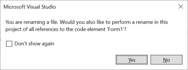
You should click the “Yes” button in order to make the renaming consistent - particularly to rename the class as well.

The Design Window

The Design Window in Visual Studio is a window used to build graphical components. To open the Design Window for a graphical component, double-click on the component’s file name in the Solution Explorer. If you are working through the example from the previous two sections, double-click “UserInterface.cs” to open its Design Window. It will initially contain a blank form:

A picture of a portion of the design window should appear here.

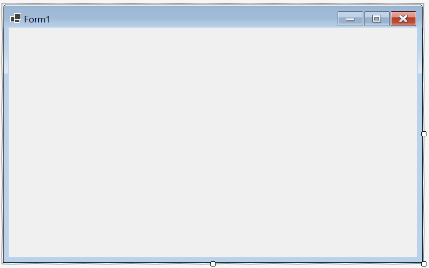
You can resize the form by dragging the handles on the right and bottom edges. You can also change the title of the form (“Form1” in the picture above) as follows:

  1. Click on the form.

  2. If the Properties window isn’t showing on the right, select “Properties Window” from the “View” menu.

  3. Look at the row of buttons near the top of the properties window, and make sure the second and third buttons are highlighted:

    A picture of a portion of a Properties window should appear here.

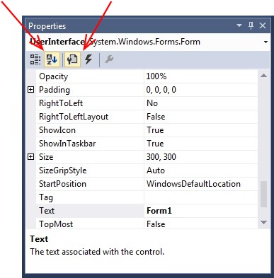
    If either of these buttons isn’t highlighted, click it to highlight it. The first two buttons on this row toggle whether the information is arranged by category (the first button) or alphabetically (the second button). The next two buttons toggle whether the control’s properties (the third button) or events (the fourth button — we’ll discuss these below) are shown.

  4. Find “Text” in the left column of the Properties window - it will probably be highlighted. Click on the space to its right, and edit the text to give your desired title. If you are working through the example, give it a title of “Hello”.

For example, after resizing and changing the title, we might have a form that looks like this:

A picture of a portion of the design window should appear here.

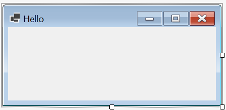
To add various graphical controls to the form, we use the Toolbox, which is normally available via a tab on the left edge (if not, you can always access it via the “View” menu). For example, let’s add a box that will contain text generated by the program. We open the Toolbox and click on the TextBox control, which can be found in the “Common Controls” section. We can then click on the design window (outside of the form) to bring it to the front, and drag an area on the form that we would like the TextBox to fill. After doing so, there will be a handle on the right and left edges to allow horizontal resizing (don’t worry about vertical resizing yet). You can also drag the TextBox to adjust its location. If you do this, as the edges of the TextBox approach the edges of the frame, struts will appear, helping you to leave an appropriate margin.

After adding a control, we usually need to customize it to some degree. To do this, click on it, then open the Properties window again. This window will now display the properties of the TextBox. The first property we will always want to change is the name of the variable that the program will use to refer to this control. This property is called “(Name)”, and will be near the top. You will need to change this name so that it follows the naming convention for controls on forms.

There are various properties that can be changed to customize the appearance and behavior of a control. For example, we can change the font of a TextBox by changing its Font property. This in turn will affect the height of the TextBox. We can prevent the user from editing it by setting its ReadOnly property to True. If we want to allow multiple lines, we can set its Multiline property to True. This in turn will add handles to the top and bottom edges so that we can adjust its height. All of the properties of a GUI control are documented in that control’s API documentation within the .NET API browser .

Thus, continuing the above example, if we modify the TextBox’s variable name to uxDisplay, its Font property to Microsoft Sans Serif, 12pt and its ReadOnly property to True, we would have the following form:

A picture of a portion of the design window should appear here.

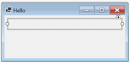
Using a similar process, we can now add a Button to the form and name it uxGo. To change the text in the Button, we will need to change its Text property. This might give us the following:

A picture of a portion of the design window should appear here.

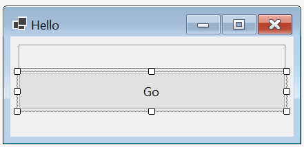
Now that we have a Button on our form, it would be appropriate to provide some functionality for that Button. Clicking on a Button signals an event to which our program may respond. In order to cause our program to respond to such an event, we need to provide an event handler for it. Because a click is the default event for a Button, we can create an event handler for this event by simply double-clicking on the Button. Doing so will open a code window containing the contents of the source code file defining the current form. Furthermore, if the name of the Button is uxGo, the following method will have been added:

private void uxGo_Click(object sender, EventArgs e)
{

}

This method will be called whenever the Button is clicked (code causing this behavior will have been automatically added to the file containing the automatically-generated code for the form). Thus, to provide the appropriate functionality for the Button we just need to add code providing this functionality to this method. We will discuss this in more detail in the next section .

Before we leave the design window entirely, however, we need to talk about a more general way of accessing the event handlers associated with controls. Going back to the Properties window for a control, clicking the fourth button in the row of buttons near the top (the one that looks like a lightning bolt) will cause all of the possible events for that control to be displayed, and any event handler that has been created for that event. For example, if we have created the event handler described above, then the list of events for the Button looks like this:

A picture of a portion of a Properties window should appear here. A picture of a portion of a Properties window should appear here.

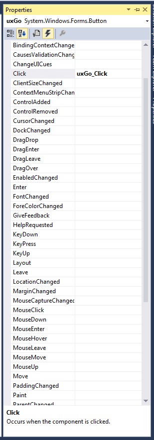
This list is useful for two reasons. The more obvious reason is that we sometimes might want to handle an event that is not the default event for a control. For example, we might want a Button to react in some way (perhaps by changing color, for example) whenever the mouse enters or leaves it. In order to implement this functionality, we would need event handlers for the MouseEnter and MouseLeave events. We can add these event handlers by double-clicking these events in this list.

The less obvious use for this list is to remove an event handler. Often we find that we have added an event handler that we don’t need, perhaps by double-clicking in the wrong place. When this happens, shouldn’t just delete the code, because there is other automatically-generated code that refers to it. Deleting the code for an event handler would therefore lead to a syntax error. Instead, the proper way to remove an event handler is to go to the list of events, right-click on the name of the event, and select “Reset” from the resulting popup menu. This safely deletes the code and all automatically-generated references to it. (Sometimes it doesn’t delete the code, but if not, it is now safe to delete it.)

The Code Window

In the previous section , we designed the following GUI:

The GUI designed in the previous section.

We also indicated briefly how functionality could be added to the button by double-clicking it in the design window to create an event handler. Creating this event handler also opens the code window to display it. The code window for this file can also be displayed by pressing F7 in the design window or by right-clicking the source code file name in the Solution Explorer and selecting “View Code”. Once a code window has been opened, it can be brought to the front by clicking the tab containing its file name near the top of the Visual Studio window. This window should look something like this:

A picture of a window should appear here. A picture of a window should appear here.

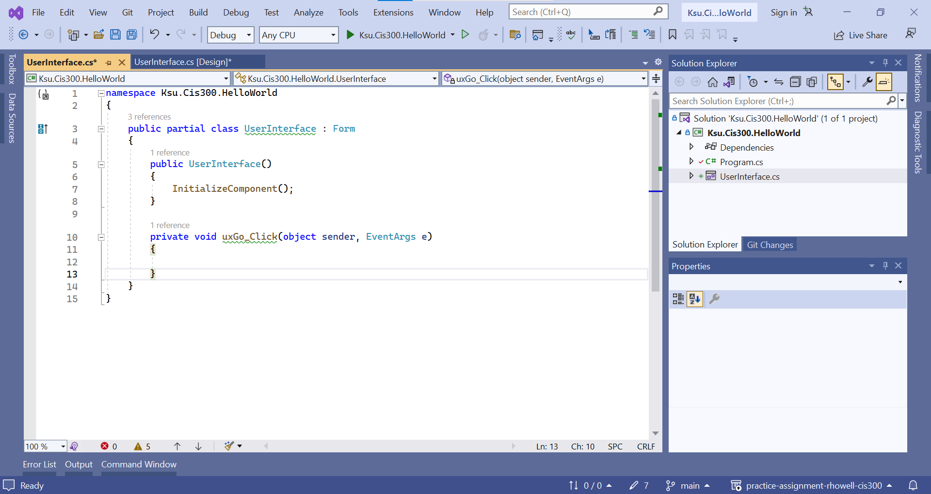
Here is a ZIP archive containing the entire Visual Studio solution . After downloading and expanding it, you may need to navigate through a folder or two, but you should be able to find a file, Ksu.Cis300.HelloWorld.sln (the “.sln” suffix may not be visible, but it should show as type “Microsoft Visual Studio Solution”). If you double-click on this file, Visual Studio 2022 should open the solution (if you have an older version of Visual Studio on your machine, you may need to right-click the file and select “Open with -> Microsoft Visual Studio 2022”).

Note in the class statement the keyword, partial. This indicates that not all of this class definition is in this file. The remainder of the definition is in the file, UserInterface.Design.cs. Recall that this file contains code for laying out the GUI and making the uxGo_Click method an event handler for the “Go” button. One of the method definitions that it contains is the InitializeComponent method, which does the layout of the GUI and sets up the event handlers. Recall also that the Main method in Program.cs constructs an instance of this class, then displays it and begins processing events for it. Because the constructor (see the code window above) calls the InitializeComponent method, everything will be set up to run the application - all that is needed is code for the event handler. This code will then be executed every time the “Go” button is clicked.

Before we add code to the event handler, let’s first take care of a couple of other issues. Note that in the code window shown above, lines 3 and 10 contain code underlined in green. These underlines indicate compiler warnings. While code containing warnings will execute, one of the requirements of CIS 300 is that all code submitted for grading be free of warnings (see Programming Style Requirements ).

We can see each warning by hovering the mouse over the underlined code. For example, hovering over “UserInterface” in line 3 displays the following:

A warning message.

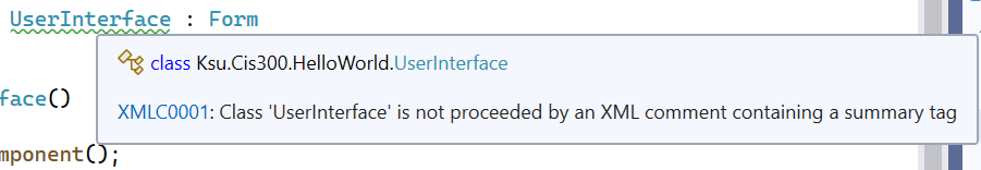
This warning refers to the CIS 300 style requirement that each class, structure, enumeration, field, property, and method be preceded by an appropriate comment (see Comments ). To remove this warning, insert a new line prior to line 3, and type /// on this new line. This will cause an XML comment to be inserted:

/// <summary>
/// 
/// </summary>
public partial class UserInterface : Form

This is not quite enough to remove the warning. To accomplish this, text must be entered between <summary> and </summary>. Any non-blank text will remove the warning, but in order for the comment to be useful, the text should summarize the purpose of the class; for example,

/// <summary>
/// A GUI for a Hello World program.
/// </summary>
public partial class UserInterface : Form

Line 10 actually contains four warnings. Three of them can be removed by adding an appropriate comment, including descriptions of the two parameters (all event handlers in CIS 300 will have similar parameter lists, though the type of the second parameter will vary depending on the type of event that is being handled):

/// <summary>
/// Handles a Click event on the "Go" button.
/// </summary>
/// <param name="sender">The object signaling the event.</param>
/// <param name="e">Information about the event.</param>
private void uxGo_Click(object sender, EventArgs e)

These, comments, however, do not take care of the last warning, which states that uxGo_Click is not in Pascal case. This refers to the naming convention for methods. To fix this warning, we need to rename this event handler by removing ux and _.

Warning

Care must be taken when renaming an identifier, as all occurrences of the identifier need to be changed. In this case, some occurrences of this name are in the automatically-generated code in UserInterface.Designer.cs. Because the Design window relies on this code, failing to change these occurrences will cause the Design window to fail to open due to syntax errors in this file.

The safe way to change any identifier name within Visual Studio is to use its Rename feature. First, right-click on the name to be changed, and select “Rename…” from the resulting popup menu. This will open a dialog within which the name can be changed. Once the name is changed, press Enter to cause the identifier to be renamed globally.

All warnings should now be gone. However, the CIS 300 style requirements specify two other comments that need to be added (see Comments ). First, an XML comment needs to be added to the constructor. Second, a comment containing the file name and the author’s name needs to be inserted at the top of the file, after inserting these comments, your code should resemble the following (with “Rod Howell” replaced by your name):

/* UserInterface.cs
 * Author: Rod Howell
 */
namespace Ksu.Cis300.HelloWorld
{
    /// <summary>
    /// A GUI for a Hello World program.
    /// </summary>
    public partial class UserInterface : Form
    {
        /// <summary>
        /// Constructs the GUI.
        /// </summary>
        public UserInterface()
        {
            InitializeComponent();
        }

        /// <summary>
        /// Handles a Click event on the "Go" button.
        /// </summary>
        /// <param name="sender">The object signaling the event.</param>
        /// <param name="e">Information about the event.</param>
        private void GoClick(object sender, EventArgs e)
        {

        }
    }
}

Now we can finally turn our attention to providing functionality to the “Go” button; i.e., we will add code to the GoClick event handler. In order for this code to provide meaningful functionality, it will need to interact with the controls on the GUI. It needs to use their variable names to do this. The name of the TextBox in this code is uxDisplay (recall that you can find this variable name by opening the design window , clicking on the control, and finding its “(Name)” property in its Properties window). Suppose we want to respond to the event by placing the text, “Hello world!”, in this TextBox. We therefore need to change its Text property to contain this string; i.e.:

private void GoClick(object sender, EventArgs e)
{
    uxDisplay.Text = "Hello world!";
}

Notice that when you type a quote mark, a matching quote is automatically added following the text cursor. As long as you don’t reposition the text cursor, you can just type the closing quote as you normally would after typing the text string — Visual Studio won’t insert another quote mark, but will move the text cursor past the one it inserted automatically. The same behavior occurs when you type open parentheses, brackets, or braces.

The code window has several features that help with code writing. One of these features is auto-completion. Often while you are typing code, an auto-complete list appears, often with an entry highlighted. When an entry is highlighted (either automatically or by your selecting it manually), pressing “Enter” or typing a code element that can’t be part of the name (such as “.” or “+”) will insert the completion into your code. Once you get used to this feature, it can greatly speed up your code entry. Furthermore, it can be a helpful reminder of what you might need to type next. If you don’t want a name to auto-complete (perhaps because it is a name you haven’t defined yet), you can press “Esc”, and the auto-complete list will disappear.

Warning

If you are not using a lab machine, you might notice that as you type text, Visual Studio often provides auto-completions for the entire line. In some cases, the auto-completion is what you need, but in other cases, it is not. This feature can speed up the code-writing process for experienced programmers who use an auto-completion when they see that it matches what they were going to type. For inexperienced programmers, however, it can actually slow both the coding process and the learning process by making bad suggestions. If you find yourself using the auto-complete suggestions as hints, it would make sense to disable them, as these “hints” are often misleading. To disable this feature:

  1. From the “Tools” menu, select “Options…”.
  2. From the list on the left, select “IntelliCode”.
  3. In the large box in the upper-right, uncheck “Show whole line completions”.
  4. Save any changes, and restart Visual Studio.

This feature has been disabled on the lab machines.

Another feature of the code window is parameter information that shows as a popup box when you are typing a parameter list in a method call; for example:

A picture of part of a code window should appear here.

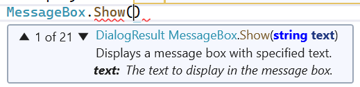
This popup box gives the return type of the method, followed by the name of the method, followed by the parameter list, with the type of each parameter shown and the current parameter in bold face. When there are more than one method with the same name, this is indicated in the upper-left corner of the popup box (“1 of 21” in the figure above — the method shown is the first of 21 methods having that name). You can use either the arrows in the popup box or the up and down arrows on the keyboard to scroll through these different methods.

A related feature allows certain information to be obtained by hovering the mouse over different code elements. For example, hovering the mouse over an identifier will display the declaration and documentation for that identifier in a popup box. Also, hovering the mouse over a syntax error (indicated by a red underline, as shown under “Show” in the above figure) will display an explanation of the error, in addition to any information on the code element.

The Debugger

In previous sections, we discussed how a Windows Forms Application can be built using Visual Studio. Having built an application, we need to be able to run and test it. To do this, we use the Visual Studio Debugger. When an application is loaded into Visual Studio, we can invoke the debugger by clicking the “Start Debugging” button near the top:

A picture of part of a Visual Studio Window should appear
here.

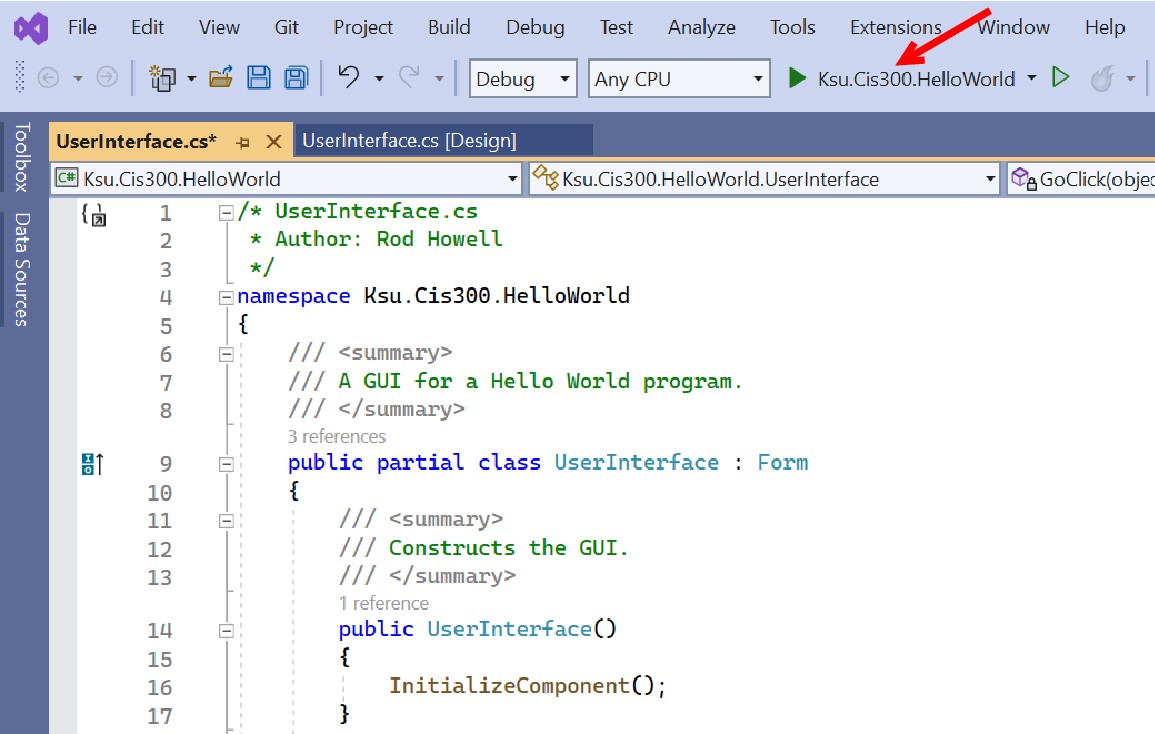
When the debugger starts, it attempts to do the following things:

  • Save any unsaved files.
  • Compile the source code into executable code.
  • Run the compiled code as an application.

If everything works correctly, the application is complete. Rarely, however, does everything work correctly the first time. Through the remainder of this section, we will discuss some of the ways the debugger can be used to find and fix errors.

One of the problems that can occur is that the compiler can fail to produce executable code because the source code contains syntax errors. When this happens, the following dialog is displayed:

A picture of a dialog should appear here. A picture of a dialog should appear here.

Usually the best thing to do at this point is to click the “No” button. This will stop the debugger and display the error list. This error list can be displayed at any time by clicking the error list button at the bottom of the Visual Studio window:

The error list button.

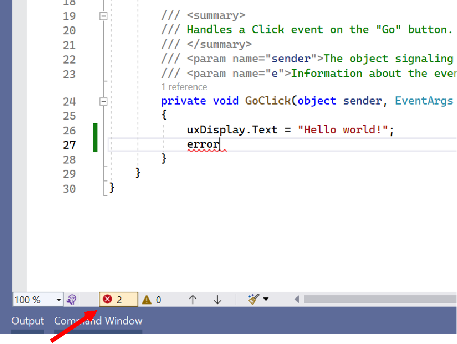
Double-clicking on a syntax error within the error list will highlight the error in the code window. Normally, fixing the error will cause the corresponding entry in the error list to disappear; however, there are times when the entry won’t disappear until the debugger is started again (i.e., by clicking the “Start Debugging” button).

Once the syntax errors are removed, the debugger will be able to generate executable code and run it. However, more problems can occur at this point. One common problem is that an exception is thrown. For example, the GitHub repository created by this invitation link (see “Git Repositories ”) contains a Visual Studio solution for a program to convert decimal numbers to base-16. Don’t worry about understanding the code, although the numerous comments may help you to do that. Instead, note that an exception is thrown when we try to convert 256:

A picture of a window should appear here. A picture of a window should appear here.

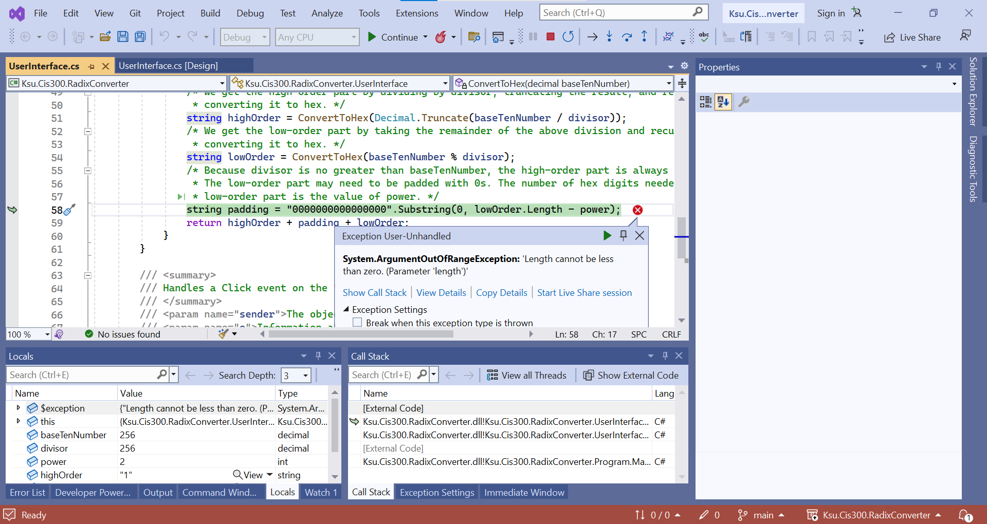
This message gives us quite a bit of information already. First, it tells us which line threw the exception - the line highlighted in green. The arrow in the left margin tells us the same thing, but more generally, when the debugger is running, it indicates the line that is currently being executed or that is ready to be executed. The popup window indicates what kind of exception was thrown: an ArgumentOutOfRangeException. It also provides the additional information that a length was less than zero when it should not have been.

Having this information, we can now use the debugger to investigate further the cause of the exception. First, in order to see the code more clearly, we might want to close the popup window (we can always get it back by clicking the red circle containing the white ‘X’). We can now examine the values of any of the variables at the time the exception was thrown by hovering the mouse over them. For example, if we hover over lowOrder, a popup appears indicating that it has a value of “0”. If we move the mouse to hover over its Length property, we can see that it has a value of 1. Hovering over power shows that it has a value of 2. Thus, we can see that the exception was thrown because we gave the Substring method a length of 1 - 2 = -1. This can be confirmed by hovering the mouse over the “-” in the expression - the popup indicates that the value of the expression is, in fact, -1.

Actually fixing the error requires a little more understanding of the code. In this case, however, the comment immediately above the line in question helps us out. It tells us that the low-order part of the hex string we are building may need to be padded with 0s - this padding is what we are constructing. Furthermore, it tells us that the number of hex digits we need is the value of power. In order to get this many digits, we need to subtract the number of hex digits we already have in lowOrder from power; i.e., we need to reverse the order of the subtraction.

To stop the debugger, notice the buttons that are available at the top of the Visual Studio window while the debugger is running:

Buttons used within the debugger.

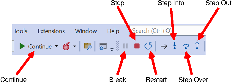
As you might guess, the “Stop” button stops the debugger. In what follows, we will discuss each of the other buttons indicated in the above figure, as well as other features of the debugger.

When debugging code, it is often useful to be able to pause execution at a particular place in order to be able to examine the values of variables as we did above. To accomplish this, we can set a breakpoint by clicking in the left margin of the code window at the line where we would like execution to pause. This places a large red dot in the margin where we clicked and colors the line red:

A picture of part of a code window should appear here. A picture of part of a code window should appear here.

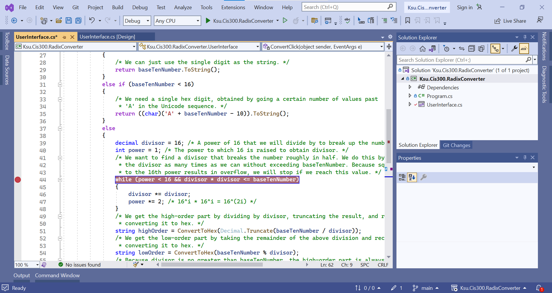
Whenever execution reaches a breakpoint, execution stops prior to executing that line. At this point, we can examine the values of variables as we described above. When we are ready to continue execution of the program, we click the “Continue” button. A breakpoint can be deleted by clicking on the red dot, or all breakpoints may be deleted by selecting “Delete All Breakpoints” from the “Debug” menu. A breakpoint may be disabled, but not deleted, by hovering over the large red dot and selecting “Disable” from the resulting popup. All breakpoints may be disabled by selecting “Disable All Breakpoints” from the “Debug” menu.

Sometimes we only want the execution to pause at a breakpoint when a certain condition is met. Such a situation might occur if we have a bug that only surfaces after the code containing it has already executed many times. Rather than letting the program stop and clicking “Continue” until we reach the point we are interested in, we can instead specify a condition on the breakpoint. To do this, right-click on the breakpoint in the left margin, and select “Conditions…” from the resulting popup menu. This causes a large box to be inserted into to the code below this line:

A picture of a Visual Studio window should appear here. A picture of a Visual Studio window should appear here.

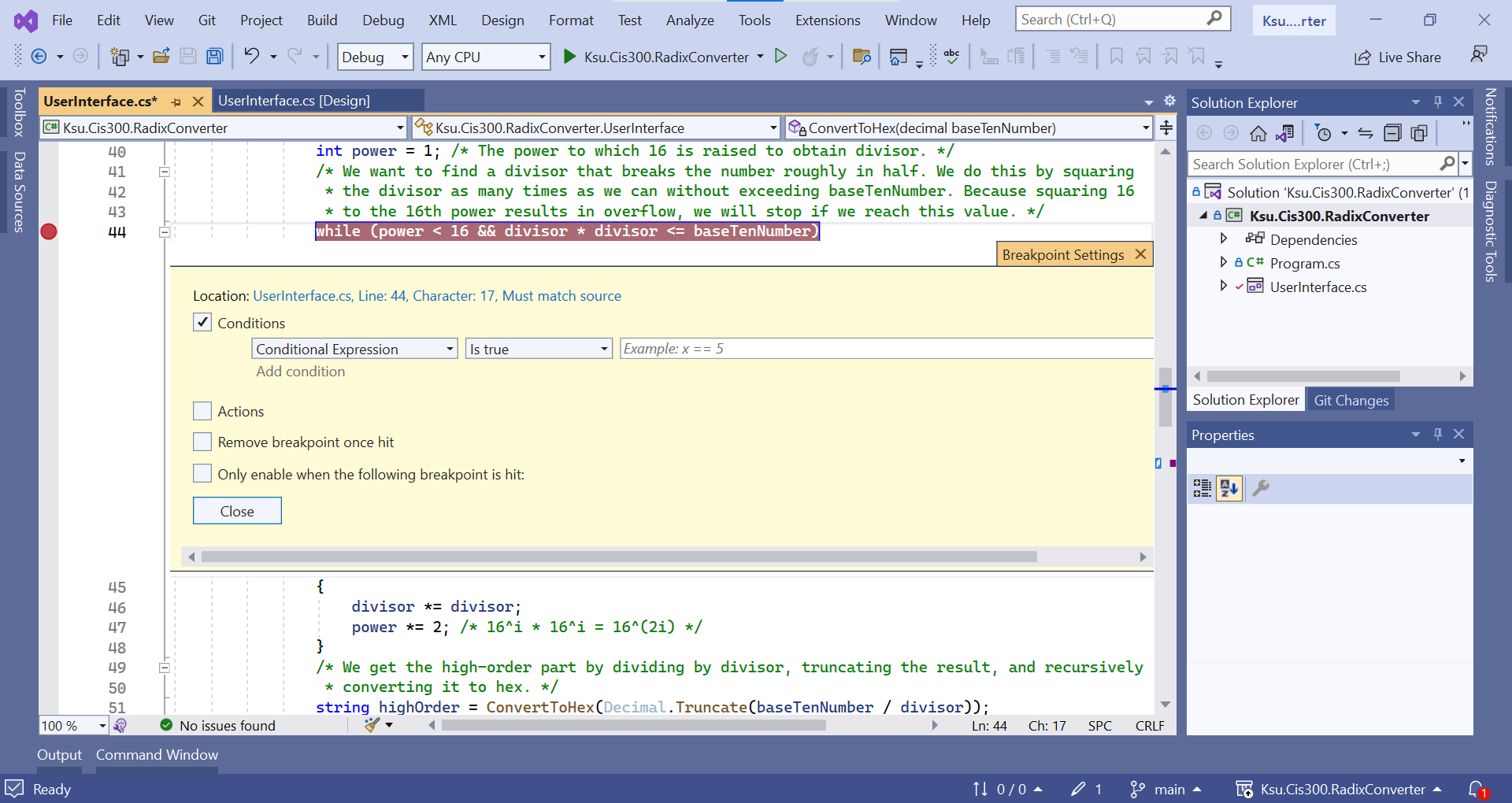
In this box, we can type an expression using variables visible at that program location. We can also choose whether we want execution to pause when that expression is true or whenever that expression has changed.

For example, we could add to the above breakpoint the condition:

power == 8

Then when we run the debugger, execution will only pause at this breakpoint when power reaches a value of 8. Note that this line is executed at the top of each iteration of the loop; hence, the breakpoint condition is checked on each iteration.

While hovering the mouse over variable names is a useful way to discover their current values, there are other mechanisms for doing this as well. For example, while the debugger is paused, you can go to the “Debug” menu and select “Windows -> Locals”. This will open a window displaying all of the local variables for the current method, property, or constructor, together with their current values. If the debugger is paused within a constructor or a non-static method or property, this window also contains this, which refers to the object that contains the constructor, method, or property. From this, you can access the non-static fields of this object.

Another mechanism for examining values of variables is through the “Immediate” window, which can also be accessed from the “Debug” menu via its “Windows” sub-menu. Within the Immediate window, you may type an expression involving the variables that are currently visible, press “Enter”, and it will display the value of that expression. This can be particularly useful when you have a large data structure, and you need to know a particular element in that structure. For example, suppose array is a large int[ ], and suppose i is an int. Using the “Locals” window, it might be rather tedious to find the value of array[i]. Using the Immediate window, however, you can just type in

array[i]

and it will display its value.

When debugging, it is often useful to be able to step through the execution of a piece of code so that you can see exactly what it is doing. Three buttons are available for this purpose: “Step Into”, “Step Over”, and “Step Out”. Suppose we were to run the code in the GitHub repository provided above with the (unconditional) breakpoint shown in the above picture, and suppose we were to enter the value, 12345. Execution will then pause at this breakpoint with divisor equal to 16 and power equal to 1. Clicking either the “Step Into” button or the “Step Over” button will cause the debugger to evaluate the loop condition and, because its value is true, advance to the “{” on the next line. We may continue to walk through the execution a step at a time using either of these buttons - as long as we are in this loop, they will have the same effect. If the Locals window is open, whenever a variable changes value, this value will be shown in red.

After one iteration, the loop will terminate, and execution will reach the line where highOrder is defined. At this point, the functionality of the “Step Into” and “Step Over” buttons becomes different because this line contains a method call. The “Step Over” button will cause execution to run normally through the method call, and pause again as soon as the method call returns (however, because this is a recursive call, if the breakpoint is still set, execution will pause when it reaches the breakpoint within the recursive call). Thus, we can see the net effect of this method call without having to walk through it a step at a time. On the other hand, we might want to step through it in order to see what it is doing. We can do this using the “Step Into” button. If at some point we want to finish executing the method we are in, but pause after it returns, we can click the “Step Out” button.

When stepping through code, a “Watch” window is often a convenient way to keep track of the value of one or more specific variables and/or expressions. You can open a Watch window from the “Debug” menu under “Windows -> Watch” — the four choices here are four different Watch windows that you may use (perhaps for debugging different parts of your program). A Watch window combines some of the advantages of the Locals window and the Immediate window. If you type in a value or expression, it will appear in the “Name” column, and if it can be evaluated in the current context, its value will be displayed in the “Value” column. Furthermore the value will be updated as the debugger executes code. You may list several values or expressions in the same Watch window, and their values will all be tracked. To delete an entry from a Watch window, right-click on it and select “Delete Watch”.

Submitting Assignments

To submit a lab or homework assignment in CIS 300, you will need to do the following steps:

  1. Commit your changes to your local Git repository. You will do this through the “Git Changes” tab in Visual Studio (if you don’t see this tab, click the icon that looks like a pencil at the bottom of the Visual Studio window). In the “Git Changes” tab, in the box that says “Enter a message <Required>”, type in a message to be associated with the changes you are committing.

    Warning

    Do not check the “Amend” box. This causes the previous commit to be changed, rather than creating a new commit. If this commit is already on GitHub, you will be unable to push your amended commit.

    Then click “Commit All”. A message at the top of the “Git Changes” tab will indicate whether the commit was successful.

  2. Push your committed changes to GitHub. Do this by clicking the up-arrow icon at the top of the “Git Changes” tab. Note that only committed changes will be pushed. A message at the top of the “Git Changes” tab will indicate whether the push was successful.

  3. Submit the URL of the commit you want graded using the submission form provided in the assignment instructions. This requires the following steps:

    • Reload the GitHub repository for this assignment in your web browser, and click on the link showing the number of commits (this is in the top right corner of the list of files and folders in the repository). This will show a list of commits, beginning with the latest. To the right of each commit is a button labeled “<>”. This button links to a web page displaying the entire contents of that commit. (It’s a good idea to check to see that all of your source code files are present, in case something went wrong.) The URL of this page will end in a 40-digit hexadecimal number giving a digital fingerprint of the commit. Copy this entire URL to the submission form at the bottom of the assignment.
    • To complete your submission, click the “Submit Assignment” button in the assignment submission form. The time at which this button was clicked will be the official submission time for your assignment.
Warning

It is important to do all three of these steps in this order. In particular, if you make any changes between your last commit and the push, these changes won’t be included in the submission. It is also important to include the correct URL.

Tip

You can double-check that all changes have been pushed by looking at the numbers next to the up-down-arrows and pencil icons at the bottom of the Visual Studio window. If all changes have been pushed, all numbers should be 0.

Occasionally, problems can occur with the interface between Visual Studio and GitHub. These problems can prevent your code from being pushed to GitHub. While the problems can often be fixed, it is often easier to bypass Visual Studio altogether, and use GitHub’s file upload mechanism.

Warning

This is not the preferred assignment submission procedure because it is less automated (and hence more error-prone), and it creates a commit on GitHub that is not in your local git repository. However, it can be used if the above procedure doesn’t work for you.

To use this alternative submission procedure, do the following steps:

  1. If Visual Studio is running, exit this application, making sure all files are saved.

  2. In your web browser, navigate to the repository for the assignment you are submitting. You should see a list of files and folders, including a file whose name ends with “.sln”.

  3. In your Windows file browser, navigate to your project folder for this assignment. You should see the same list of files and folders as is shown in your web browser. (Depending on the settings for your local machine, you may not see file name suffixes such as “.sln” and “.gitignore”, and if you’ve added any projects that were not in the original repository, their folders may be shown in the file browser but not in the web browser.)

  4. In your web browser, click the “Add file” button in the row of buttons above the list of files and folders, and select “Upload files” from the drop-down menu.

  5. In your file browser, type Control-“A” to select all files and folders, and drag them to the web browser where it says, “Drag files here …”. The web browser should indicate a number of files being uploaded.

  6. Near the bottom of the web browser window, in the text box below “Commit changes”, type a commit message, then click the “Commit changes” at the bottom. It may take a little while to process, but eventually you should see the repository again.

  7. Make sure all of your “.cs” files are present in the GitHub repository, and that they contain the code you want. (If you have removed or renamed any files, the original files may still be in the repository; however, they shouldn’t be in the solution, and therefore shouldn’t interfere with the program’s execution.)

  8. Submit the URL of this commit by following Step 3 of the assignment submission process given above.

Unit Testing

Some of the lab assignments in CIS 300 use a technique called unit testing for testing the correctness of your code. Unit testing is an automated technique for testing individual public methods and properties using a pre-defined set of test cases. We will be using an open-source unit-testing framework called NUnit .

An NUnit test suite is a separate project contained within the same solution as the project it is to test. The GitHub repositories for lab assignments that utilize unit testing will initially contain these projects, whose names will typically end with “.Tests”. You should not modify these test projects.

A test project will contain one or more classes having the attribute, [TestFixture]. These classes will contain the specific tests, each of which is a method with the attribute, [Test]. The name of the method will briefly describe the test, and a more detailed explanation will be provided in comments.

To run the tests, first go to the “Test” menu and select “Test Explorer”. This will open the Test Explorer, which should resemble the following:
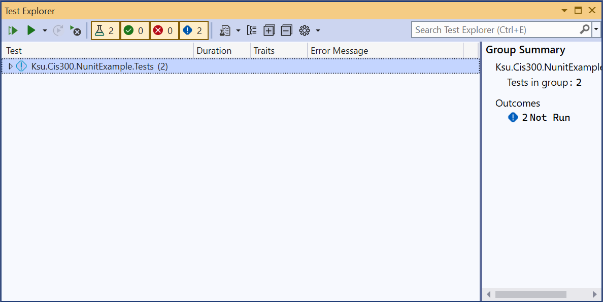
A picture of the Test Explorer should appear
here. A picture of the Test Explorer should appear
here.

Note

Depending on whether the test project has been successfully compiled, the tests in the large panel may or may not be shown.

Then click the “Run All Tests in View” button in the upper-left corner of the Test Explorer. The Test Explorer should then show the results of all the tests:
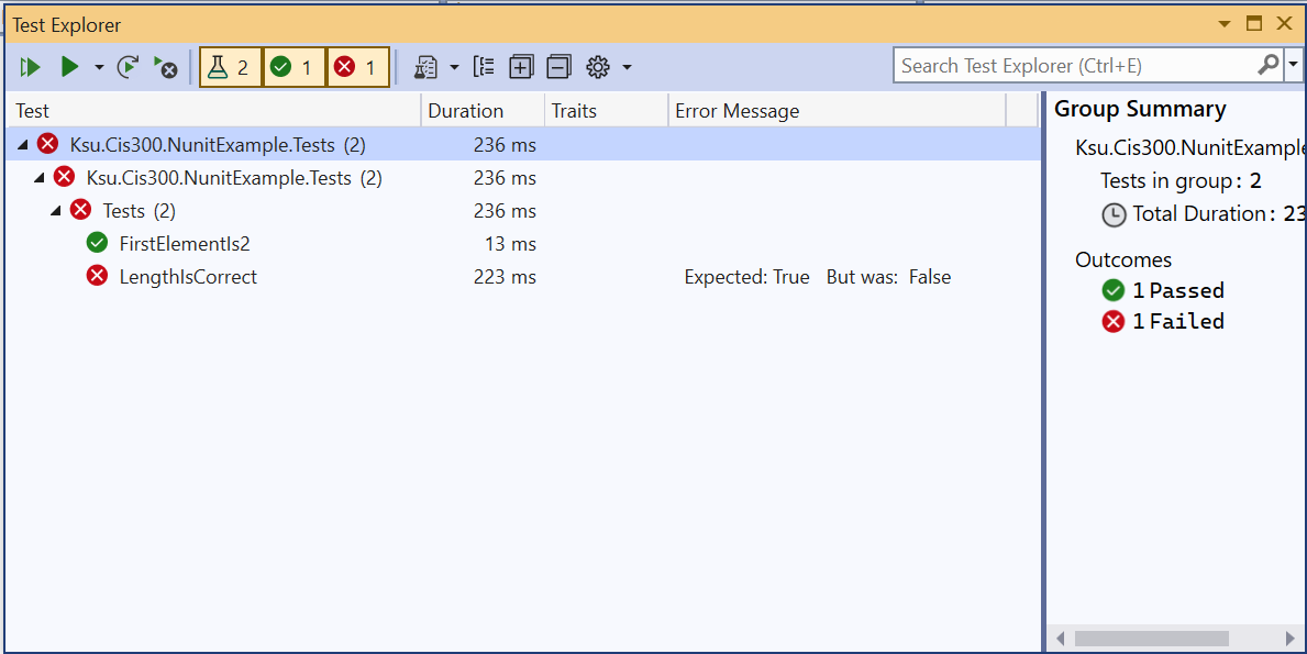
A picture of the Test Explorer should appear here. A picture of the Test Explorer should appear here.

Note

To see all of the output, you will need to open all of the elements either by clicking on the small triangles to the left of each element or by clicking the icon containing the ‘+’ symbol.

The above output shows that there were two tests in the test suite. The names of the tests are simply the names of the methods comprising the tests. The output further shows that one of the tests, LengthIsCorrect, failed, whereas the other test, FirstElementIs2, passed.

The goal, of course, is to get all the tests to pass. When a test fails, you will first want to refer to the comments on the test method in order to understand what it is testing. Then by clicking on the failed test in the Test Explorer, you can see exactly what failed in the test - this will appear in the panel on the right. In some cases, an unexpected result will have been produced. In such cases, the message will show what result was expected, and what it actually was. In other cases, an exception will have been thrown. In such cases, the exception will be displayed. A stack trace will also be displayed, so that you can tell what line of code threw the exception. Finally, you can run the debugger on the test itself by right-clicking on the test and selecting “Debug”. This will allow you to debug your code using the techniques describe in the section, “The Debugger” .

Tip

You can dock the Team Explorer into the main Visual Studio window by clicking on the small triangle in the far upper-right corner of the window and selecting either “Dock” or “Dock as Tabbed Document”.

One potential error deserves special mention. Sometimes code will throw an exception that cannot be caught by a try-catch block. By far the most common of these exceptions is the StackOverflowException. When this exception is thrown during unit testing, the test explorer will simply show some or all of the tests in gray letters. This indicates that these tests were not completed. To see why the tests were not completed, you can open the “Output” window from the “View” menu and change the drop-down menu at the top to “Tests”. This will indicate what error stopped the tests; for example, the following indicates that a StackOverflowException has occurred:

A picture of an output window should appear here. A picture of an output window should appear here.

Unfortunately, when this error occurs, it’s more difficult to determine which test caused the exception. You can run the debugger on each test individually to see if it throws a StackOverflowException. In many cases, however, it is easier to examine each recursive call to make sure the call is made on a smaller problem instance.

When you believe you have fixed any errors in your code, you will usually want to run all the tests again, as fixing one error can sometimes introduce another. However, there are times, such as when some of the tests are slow, when you don’t want to run all the tests. In such cases, you can select an appropriate alternative from the “Run” drop-down at the top of the Test Explorer (i.e., from the drop-down button with the single green triangle on it). A useful option from this menu is “Run Failed Tests”. Alternatively, you can select one or more tests from the Test Explorer (use Ctrl-Click to select multiple tests), then right-click and select “Run”.

Whenever you run fewer than all the tests, the tests that were not run are dimmed in the Test Explorer to indicate that these results are not up to date. Be sure you always finish by running all the tests to make sure they all pass on the same version of your code.

Each CIS 300 lab assignment that uses unit testing is set up to use GitHub’s auto-grading feature, so that whenever the assignment is pushed, the server will run the unit tests. The overall result of the tests is indicated by an icon on the line below the “<> Code” button on the repository’s web page (you may need to refresh the page to show the latest commit). A brown dot indicates that the tests have not yet completed (this usually take a couple of minutes). A green check mark indicates that all tests have passed. A red X indicates that at least one test has failed, or that the tests couldn’t be run.

Unit testing will not be done by the GitHub server on any homework assignments in CIS 300. Instead, the auto-grading feature is used for a different purpose - to record push times. Thus, each push will result in an indication that all tests have passed, even if the code doesn’t compile.

You may receive emails indicating the results of auto-grading. You can control this behavior as follows:

  1. On any GitHub page, click on the icon in the upper-right corner and select “Settings”.
  2. On the navigation pane on the left, click “Notifications”.
  3. Scroll down to the “System” section, and select your desired notification behavior under “Actions”.

Using Multiple Machines

Source control provides one way to access your code from multiple machines. Before you decide to do this, however, you should consider whether this is the best approach. For example, if you have a CS Account , you have a network file system (the U: drive on CS Windows systems) that you can use whenever you have internet access. From off campus, you need to tunnel into campus using a Virtual Private Network, or VPN (see the KSU Information Technology Services page on Virtual Private Networking for instructions). Once on campus, you can mount this file system as a network drive by following the instructions on the CS support page, “DiskUsage ”.

As an alternative to the U: drive or some cloud service, you can use your GitHub repositories to store a master copy of each assignment, and clone local copies as needed on the different machines you use. Once you have code in a GitHub repository, you can clone that repository to a local machine as described in “Git Repositories ”. When you are finished working on that machine, commit all changes and push them to GitHub. If at some later point you need to resume working on a machine whose Git repository is out of date, you can update it by clicking the down-arrow icon in the Visual Studio “Git Changes” tab.

If you are careful about pushing all changes to GitHub and updating each local copy whenever you begin working on it, everything should go smoothly. Problems can occur, however, if you have made changes to a local version that is out of date, then either try to update it by pulling the GitHub copy, or try to push these changes to GitHub. In such cases, the following message will be shown:

An error message should appear here.

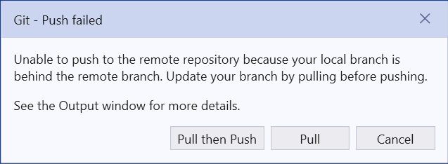
At this point, you should click the “Pull then Push” button in the above message. This usually won’t fix the problem, as indicated by an error message at the top of the “Git Changes” tab. In order to resolve the conflicts in the two versions, look in the “Unmerged Changes” section of the “Git Changes” tab. This will list the files that are different in the two versions. To resolve the conflicts in a file, right-click on it, and select “Merge…”. Visual Studio will then show the two versions of the file side by side with the conflicts highlighted. If you want the version you are currently trying to push, simply click the “Take Current” button at the top. Otherwise, you can select individual portions from the two versions - the result will be shown below the two versions. When you are satisfied with the result, click the “Accept Merge” button. Once you have merged all conflicting files, you will then need to commit and push again.

Checkpointing

Sometimes when writing code, we see that we have gone down a wrong path and would like to undo some major changes we have made. Source control can help us with this if we checkpoint by committing our changes from time to time, using commit messages that clearly describe the changes made in that commit. (Note that it is not necessary to push these commits to GitHub until you are ready to submit the assignment.) Git’s revert feature allows us to undo any of these commits.

Before you access Git’s revert feature, you should undo any uncommitted changes. To do this, go to the “Git Changes” tab, right-click on the first line under “Changes”, and select “Undo Changes”. You will be asked to confirm this action. This will undo any changes to that folder. If you have more folders containing changes, repeat this process for each changed folder.

To access Git’s revert feature, select “View Branch History” from the “Git” menu. This will reveal a list of all the commits for this local Git repository, with the most recent commit listed at the top. To undo all of the changes in any commit, right-click on that commit, and select “Revert” from the popup menu. The result is automatically committed.

Warning

You should always revert commits starting with the most recent and working backwards (i.e., from the top of the list toward the bottom). Otherwise, you will probably encounter conflicts that need to be resolved, as described in the previous section . You may even reach a state in which no commits can be reverted.

Programming Style Requirements

Software companies typically have programming style requirements to which their programmers must adhere. Many of these requirements have become industry standards. These requirements help to make the developed code more readable, portable, and maintainable. This appendix contains a short set (much shorter than what is typically found in industry) of programming style requirements for CIS 300. These requirements are consistent with Microsoft’s Naming Guidelines and de facto industry accepted practices. Other requirements are simplifications introduced due to the fact that this programming is for course assignments, rather than for distribution. All assignments in CIS 300 use the package KSU.CS.CodeAnalyzers to assist with meeting many of these requirements. This package will generate warnings when various style requirements are violated. All code submitted for grading is expected to follow these style requirements and to be free of warnings.

Subsections of Programming Style Requirements

General Formatting

All programming will be done using Microsoft Visual Studio® Community 2022 . This integrated development environment (IDE) does a certain amount of formatting automatically. All code formatting should be consistent with what the IDE does automatically, including how it formats code stubs that it inserts. Specifically, all braces should occur on lines by themselves, vertically aligned so that matching braces occupy the same column. (An exception to this rule can be made when the braces enclose a single statement or a part of a statement, and they occur on the same line; however, if it is possible to omit the braces, as in an if statement, this is preferable to placing them on the same line.) Furthermore, blocks of code enclosed by braces should be indented one tab stop inside the braces.

Tip

An easy way to format a file consistently (after removing any syntax errors) is to select from the “Edit” menu, “Advanced -> Format Document”.

Warning

Don’t change the formatting defaults in the IDE.

Access Modifiers

C# provides 4 access modifiers for classes, fields, etc.: public, internal, protected, and private. For simplicity, however, we will not allow the use of the internal or protected access modifiers unless they are required by the compiler (for example, when overriding a protected method).

When classes, fields, etc., are declared, C# does not require that an access modifier be used. If the access modifier is omitted, a default accessibility level will be used. However, the default depends on where it is being declared. For example, the default accessibility level of a top-level type is internal, whereas the default accessibility level of a class member is private. In order to avoid confusion, we will require that access modifiers (i.e., public or private) be used on all declarations except where C# does not allow them (C# does not allow access modifiers for namespaces, members of interfaces or enumerations, or local variables within methods). In particular, note that when Visual Studio® automatically generates a class statement, it does not always supply an access modifier, or it may use internal. We require that the statement be changed to use public (C# does not allow private here).

In addition, fields within classes and structures should be declared private, unless they are also declared either const or readonly . If you want to make a variable accessible to outside code, you can instead do something like the following:

public double Force { get; set; }

Or if you want the outside code to be able to access it, but you don’t want it to change its value you can instead define it as:

public double Force { get; private set; }

In these examples, Force is not a field, but a property . It can be used like a field, but defining it as a property makes it more maintainable (see “Properties” for more details).

Warning

Don’t define a private property when a private field will accomplish the same thing - using a private field with the appropriate naming convention makes the code more readable.

For more information on access modifiers and accessibility levels, see the section on Accessibility Levels in the C# Reference .

Naming Conventions

The naming conventions described below use the following terminology:

  • Pascal case: Multiple words are joined without spaces, using capital letters at the beginning of each word. If acronyms of 3 or more letters are included, only the first letter of the acronym is capitalized. For example, AverageAge, ContextBoundObject, RgbCode.
  • Camel case: The same as pascal case, except the first letter is not capitalized. For example, averageAge, contextBoundObject, rgbCode.

Namespaces

In CIS 300 programming assignments, namespace names will typically be provided. They will use the form Ksu.Cis300.ProgramName, where each of the 3 components is in pascal case. For example:

namespace Ksu.Cis300.Spreadsheet
{

}

Classes, Structures, and Enumerations

Use pascal case. If the name begins with “I”, the following letter must not be capitalized, as this would look like an interface - see below. For an exception class, append the word “Exception”. Make your names descriptive nouns or noun phrases without abbreviations (common abbreviations like “Min” are allowed). For example:

public class AccountManager
{

}

Interfaces

Use the convention for a class name with a capital “I” preceding the first letter (which must also be capitalized). For example:

public interface IPriorityQueue
{

}

Methods

Use pascal case. Make your names descriptive without abbreviations (common abbreviations like “Min” are allowed). For example:

private void InitializeComponent()
{

}
Warning

Automatically-generated event handlers don’t follow this convention. For example, suppose you generate a Click event handler by double-clicking a Button named uxUpdate. The event handler generated will then be given a name of uxUpdate_Click. You will need to rename it to UpdateClick. Be sure to use Visual Studio’s Rename feature , as this name will also need to be changed in automatically-generated code that you normally won’t edit.

Properties

Use pascal case. Make your names descriptive without abbreviations (common abbreviations are allowed). For example:

public int Count { get; private set; }

Controls on Forms

Use camel case, and begin names with “ux” followed by a capital letter (this “ux” stands for “user experience”). Make your names descriptive of the functionality, not the type of control. For example, uxAccept, uxCustomerName.

Note

You will not typically declare these names in code, but will enter them in the Visual Studio® design window.

public Constants (const or readonly)

Use pascal case. Make your names descriptive. For example:

public const double GravitationalAcceleration = 9.80665;

private Fields

Use camel case with an underscore character preceding the first letter. For example:

private double _weight;

This applies to all private fields, including those defined as const or readonly.

Parameters and Local Variables Within Methods

Use camel case. For example, inString and outString in the following code:

public string ToMixedCase(string inString)
{
    string outString;
    // code here
    return outString;
}

Comments

Within each source code file that you edit, you will need to provide certain comments as documentation. Visual Studio® automatically generates some source code files that you will not need to modify — you don’t need to add comments to those files.

At the top of each file in which you provide code, add a comment of the following form:

/* filename.cs
 * Author: Name 
 */

where filename.cs is the name of the file, and Name is the name of the primary author. The primary author will either be you or, for files provided for you, the name of the original author of that file. Whenever you use someone else’s code, it is important that you give them credit for it. (To fail to do this is plagiarism.) Thus, if one of your source files was originally written by Rod Howell, leave his name as the author. If you have modified a file originally written by someone else, below the Author line, insert a line of the following form:

/*
 * Modified by: Your Name
 */

Prior to each class, structure , enumeration , field, property , and method, place a comment documenting its use. This comment should be delimited by /// on each line. When you type /// immediately above a class, structure, enumeration, field, property, or method, the IDE will automatically insert additional text to form a comment stub such as:

/// <summary>
/// 
/// </summary>

<summary> and </summary> are XML tags, which are understood by the IDE. Between these tags, you should insert a summary of the program component you are documenting, including any requirements that must be satisfied by the calling code in order for the method to work properly. For example:

/// <summary>
/// Indicates whether this structure is empty.
/// </summary>
private bool _isEmpty;

If the program component being documented is a method with at least one parameter and/or a non-void return type, additional XML tags will be generated by the IDE. For each parameter, <param> and </param> tags will be generated. You should insert a description of the use of that parameter between these tags. If the method has a non-void return type, <returns> and </returns> tags are generated. You should insert an explanation of the value being returned between these tags. For example:

/// <summary>
/// Computes the number of times a given string x
/// occurs within a given string y.
/// </summary>
/// <param name="x">The string being searched for.</param>
/// <param name="y">The string being searched.</param>
/// <returns>The number of occurrences of x in y.</returns>
private int Occurrences(string x, string y)
{

}
Note

You do not need to fill in <exception> tags - you may remove any that are generated automatically.

Visual Studio often generates warnings when it cannot verify that the value being assigned to a non-nullable variable is not null. In cases where you can determine that the value will not be null, you are allowed to remove the warning by inserting ! after the value. In such cases, prior to this line, insert a comment explaining why this value is not null. For example:

string line;
while (!input.EndOfStream)
{
    // Because input isn't at the end of the stream, ReadLine won't return null.
    line = input.ReadLine()!;
}

Comments should also be used within methods to explain anything that is not obvious from the code itself.

Prohibited Features

The following features of C# should not be used on assignments or quizzes unless otherwise stated:

  • The goto statement: It has been over 50 years since Dijkstra published “Go To Statement Considered Harmful” (Communications of the ACM, vol. 11 (1968), pp. 147-148). I am amazed that languages continue to include this statement.

  • The unsafe keyword: The name pretty much says it all.

  • The var keyword: There are very few contexts in which this is needed, and these contexts won’t occur in this class. For all other contexts, it makes the code less readable.

  • Virtual methods: These are useful in large-scale software development; however, they are overused. They will not be needed in the programming we will be doing. (However, virtual methods in the .NET class library may be overridden .)

  • Abbreviated constructor calls: Beginning with C# version 9.0, constructor calls are allowed to be abbreviated when the compiler can determine from the context the type of object that is being constructed. In such a case, the type name can be omitted from the new operator. For example, instead of writing:

    StringBuilder sb = new StringBuilder();

    we can write:

    StringBuilder sb = new();

    If the constructor takes parameters, they can be inserted between the parentheses. Such abbreviations are permitted - even encouraged - in cases like the above example, where the type being constructed is explicitly specified elsewhere in the same statement. However, if the type name is not explicitly specified elsewhere in the same statement, such abbreviations are prohibited, as they make the code harder to read.