Introduction to Trees
Introduction to Trees
A tree is a mathematical structure having a hierarchical nature. A
tree may be empty, or it may consist of:
- a root, and
- zero or more children, each of which is also a tree.
Consider, for example, a folder (or directory) in a Windows file system.
This folder and all its sub-folders form a tree — the root of the tree
is the folder itself, and its children are the folders directly
contained within it. Because a folder (with its
sub-folders) forms a tree, each of the sub-folders directly contained
within the folder are also trees. In this example, there are no empty
trees — an empty folder is a nonempty tree containing a root but no
children.
Note
We are only considering actual folders,
not shortcuts, symbolic links, etc.
We have at least a couple of ways of presenting a tree graphically. One
way is as done within Windows Explorer:
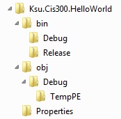
Here, children are shown in a vertically-aligned list, indented under
the root. An alternative depiction is as follows:
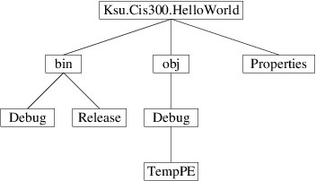
Here, children are shown by drawing lines to them downward from the
root.
Other examples of trees include various kinds of search spaces. For
example, for a chess-playing program, the search for a move can be
performed on a game tree whose root is a board position and whose
children are the game trees formed from each board position reachable
from the root position by a single move. Also, in the sections that
follow, we will consider various data structures that form trees.
.NET provides access to the folders in a file system tree
via the
DirectoryInfo
class, found in the System.IO namespace. This class has a
constructor
that takes as its only parameter a string giving the path to a
folder (i.e., a directory) and constructs a DirectoryInfo describing
that folder. We can obtain such a string from the user using a
FolderBrowserDialog
.
This class is similar to a file
dialog
and can be added
to a form in the Design window in the same way. If uxFolderBrowser is
a FolderBrowserDialog, we can use it to obtain a DirectoryInfo
for a user-selected folder as follows:
if (uxFolderBrowser.ShowDialog() == DialogResult.OK)
{
    DirectoryInfo folder = new(uxFolderBrowser.SelectedPath);

	// Process the folder
}
Various properties of a DirectoryInfo give information about the
folder; for example:
- Name
gets the name of the folder as a string.
- FullName
gets the full path of the folder as a string.
- Parent
gets the parent folder as a DirectoryInfo?. If the current folder is the root of its file system, this property is null.
In addition, its
GetDirectories
method takes no parameters and returns a DirectoryInfo[ ] whose
elements describe the contained folders (i.e., the elements of the array
are the children of the folder). For example, if d refers to a
DirectoryInfo for the folder Ksu.Cis300.HelloWorld from the
figures above, then d.GetDirectories() would return a 3-element
array whose elements describe the folders bin, obj, and
Properties. The following method illustrates how we can write the
names of the folders contained within a given folder to a
StreamWriter
:
/// <summary>
/// Writes the names of the directories contained in the given directory
/// (excluding their sub-directories) to the given StreamWriter.
/// </summary>
/// <param name="dir">The directory whose contained directories are to
/// be written.</param>
/// <param name="output">The output stream to write to.</param>
private void WriteSubDirectories(DirectoryInfo dir, StreamWriter output)
{
    foreach (DirectoryInfo d in dir.GetDirectories())
    {
        output.WriteLine(d.Name);
    }
}
For a more interesting problem, suppose we want to write to a
StreamWriter the structure of an entire folder, as follows:
Ksu.Cis300.HelloWorld
  bin
    Debug
    Release
  obj
    Debug
      TempPE
  Properties
We can break this task into the following steps:
-
Write the name of the folder:
Ksu.Cis300.HelloWorld
-
Write the structure of each child folder, indented one level (i.e.,
two spaces):
-
First child:
  bin
    Debug
    Release
-
Second child:
  obj
    Debug
      TempPE
-
Third child:
Properties
Note that writing the structure of a child
folder is an instance of the original problem that we want to solve -
i.e., writing the structure of a folder. The only difference is that the
folders are different and the amount of indentation is different. We can
solve such a problem using a technique called recursion. Recursion
involves a method calling itself. Because of the recursive nature of a
tree (i.e., each child of a tree is also a tree), recursion is commonly
used in processing trees.
In order to use recursion, we first must define precisely what we want
our method to accomplish, wherever it might be called. For this problem,
we want to write to a given StreamWriter a list of all the folders
contained within a given folder, including the given folder itself and
all sub-folders in the entire tree, where each folder is indented two
spaces beyond its parent’s indentation. Furthermore, the entire tree
below a given folder (i.e., excluding the folder itself) should be
listed below that folder, but before any folders that are outside that
folder. In order to write such a method, we need three parameters:
- a DirectoryInfo giving the root folder;
- a StreamWriter where the output is to be written; and
- an int giving the level of indentation for the root folder,
where each level of indentation is two spaces.
Because the root folder must be written first, we begin there. We first
must write two blanks for every level of indentation, then write the
name of the root folder:
/// <summary>
/// Writes the directory structure for the given root directory to the
/// given StreamWriter, indenting all entries to the given indentation
/// level (incomplete).
/// </summary>
/// <param name="root">The root directory.</param>
/// <param name="output">The output stream to which to write</param>
/// <param name="level">The current indentation level.</param>
private void WriteTree(DirectoryInfo root, StreamWriter output, int level)
{
    for (int i = 0; i < level; i++)
    {
        output.Write("  ");
    }
    output.WriteLine(root.Name);

    // We now need to write the sub-directories . . .

}
We can get the children using root.GetDirectories(). Each of the
elements of the array this method returns will be a DirectoryInfo
whose structure we want to write. Looking back at how we described what
we want the WriteTree method to accomplish, we see that it is
exactly what we want to do for each child. We can therefore make a
recursive call for each child, specifying that the indentation level
should be one deeper than the level for root:
/// <summary>
/// Writes the directory structure for the given root directory to the
/// given StreamWriter, indenting all entries to the given indentation
/// level (incomplete).
/// </summary>
/// <param name="root">The root directory.</param>
/// <param name="output">The output stream to which to write</param>
/// <param name="level">The current indentation level.</param>
private void WriteTree(DirectoryInfo root, StreamWriter output, int level)
{
    for (int i = 0; i < level; i++)
    {
        output.Write("  ");
    }
    output.WriteLine(root.Name);
    foreach (DirectoryInfo d in root.GetDirectories())
    {
        WriteTree(d, output, level + 1);
    }
}
This method accomplishes the desired task, provided the directory tree
does not contain symbolic links or anything similar that might be
represented using a DirectoryInfo, but is not an actual folder.
While it is possible to detect these and avoid following them, we will
not consider that here.
There is something that may seem mysterious about what we have done. In
order to convince ourselves that this method is written correctly, we
need to know that the recursive calls work correctly; however, the
recursive calls are to the same method. Our reasoning therefore seems
circular. However, we are actually using a mathematical principle from
the discipline of formally proving software correctness: in order to
prove that a recursive method meets its specification we may assume that
any recursive calls meet that same specification, provided that these
recursive calls are all on smaller problem instances.
The restriction that recursive calls are on smaller problem instances is
what avoids circular reasoning regarding recursion. We associate with
each problem instance a nonnegative integer describing its size. For a
problem involving a tree, this size is typically the number of nodes
in the tree, where a node is a root of some subtree. Because every node
in a child is also in the tree containing the child, but the root of the
containing tree is not in the child, a child is always smaller, provided
the tree is finite. (For directory trees, if the underlying file system
is a Windows system, the tree will be finite; however if it is a
non-Windows system, the trees may appear to Windows as being infinite -
the above method actually will not work in such cases.)
The validity of this strategy is based on the fact that for any method,
the following three statements cannot be simultaneously true:
- All of the method’s recursive calls (if there are any) are on inputs
of smaller size, where the size is defined to be a nonnegative
integer.
- When the method is given any input, if all of the method’s recursive
calls produce correct results, then the method itself produces a
correct result.
- There is at least one input for which the method does not produce a
correct result.
Thus, if we can ensure that Statements 1 and 2 are true, then Statement
3 must be false; i.e., the method will be correct. To ensure Statement
2, we only need to concern ourselves with cases in which all recursive
calls produce correct results; hence, we simply assume that each
recursive call produces correct results.
To see why the three statements above cannot be simultaneously true,
let’s first suppose Statement 3 is true. Let S be the set of all
inputs for which the method does not produce a correct result. Then
because Statement 3 is true, this set is nonempty. Because each input in
S has a nonnegative integer size, there is an input I in S with
smallest size. Now suppose Statement 1 is true. Then when the method is
run on input I, each of the recursive calls is given an input smaller
than I; hence, because I is a smallest input in S, none of these
inputs is in S. Therefore, each of the recursive calls produces a
correct result. We therefore have an input, I on which all of the
method’s recursive calls produce correct results, but the method itself
does not produce a correct result. Statement 2 is therefore false.
Once we understand this strategy, recursion is as easy to use as calling
a method written by someone else. In fact, we should treat recursive
calls in exactly the same way — we need to understand what the recursive
call is supposed to accomplish, but not necessarily how it accomplishes
it. Furthermore, because processing trees typically involves solving the
same problem for multiple nodes in the tree, recursion is the natural
technique to use.
A recursive method for processing a tree will break down into cases,
each fitting into one of the following categories:
- A base case is a case that is simple enough that a recursive call
is not needed. Empty trees are always base cases, and sometimes
other trees are as well.
- A recursive case is a case that requires one or more recursive
calls to handle it.
A recursive method will always contain cases of both these types. If
there were no base cases, the recursion would never terminate. If there
were no recursive cases, the method wouldn’t be recursive. Most
recursive methods are, in fact, structured as an if-statement, with
some cases being base cases and some cases being recursive cases.
However, for some recursive methods, such as WriteTree above, the
base cases aren’t as obvious. Note that in that method, the recursive
call appears in a loop; hence, if the loop doesn’t iterate (because the
array returned is empty), no recursive calls are made. Furthermore, if
the directory tree is finite, there must be some sub-directories that
have no children. When the GetDirectories method is called for such
a directory, it returns an empty array. These directories are therefore
the base cases.
The WriteTree method above is actually an example of processing an
entire tree using a preorder traversal. In a preorder traversal, the
root of the tree is processed first, then each of the children is
processed using a recursive call. This results in each node’s being
processed prior to any node contained in any of its children. For the
WriteTree method, this means that the name of any folder is written
before any folders contained anywhere within it.
When debugging a recursive method, we should continue to think about it
in the same way — that is, assume that all recursive calls work
correctly. In order to isolate an error, we need to find an instance
that causes an error, but whose recursive calls all work correctly. It
will almost always be possible to find such a case that is small — in
fact, small cases tend to be the most likely ones to fit this
description. When debugging, it therefore makes sense to start with the
smallest cases, and slowly increase their size until one is found that
causes an error. When using the debugger to step through code, first
delete all breakpoints from this method, then use Step
Over
to step over
the recursive calls. If a recursive call doesn’t work correctly, you
have found a smaller instance that causes an error — work on that
instance instead. Otherwise, you can focus on the top-level code for the
instance you are debugging. This is much easier to think about that
trying to work through different levels of recursion.
There are times when it is useful to know exactly what happens when a
recursive call (or any method call, for that matter) is made. Prior to
transferring control to the top of the method being called, all local
variables and the address of the current code location are pushed onto
the call stack. This call stack is just like any other stack, except
that it has a smaller amount of space available to it. You can, in fact,
examine the call stack when debugging — from the “Debug” menu, select
“Windows -> Call Stack”. This will open a window
showing the contents of the call stack. The line on top shows the line
of code currently ready for execution. Below it is the line that called
the current method, and below that line is the line that called that
method, etc. By double-clicking on an entry in the call stack, you can
use the other debugging tools to examine the values of the local
variables for the method containing that line of code. If this method is
recursive, the values displayed for the local variables are their values
at that level of recursion.
Note
This only applies to the values
stored in local variables - in particular, if a local variable is a
reference type
, the
value of the object to which it refers will not revert to its earlier
state. For example, if a local variable is an array, the debugger will
show the value of this variable to refer to the array that it referred
to at that point, but the values shown in that array will be its current
values.
One consequence of method calls using a call stack with limited space
available is that moderately deep recursion can fill up the call stack.
If this happens, a StackOverflowException will be thrown. Thus,
infinite recursion will always throw this exception, as will recursion
that is nested too deeply. For this reason, it is usually a bad idea to
use recursion on a linked
list
- if the list is
very long, the recursion will be nested too deeply. We must also take
care in using recursion with trees, as long paths in a tree can lead to
a StackOverflowException. Due to the branching nature of trees,
however, we can have very large trees with no long paths. In fact, there
are many cases in which we can be sure that a tree doesn’t contain any
long paths. In such cases, recursion is often a useful technique.
Subsections of Binary Search Trees
Binary Trees
Binary Trees
A binary tree is a tree in which each node has exactly two children,
either of which may be empty. For example, the following is a binary
tree:
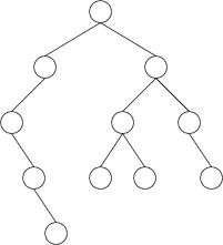
Note that some of the nodes above are drawn with only one child or no
children at all. In these cases, one or both children are empty. Note
that we always draw one child to the left and one child to the right. As
a result, if one child is empty, we can always tell which child is empty
and which child is not. We call the two children the left child and
the right child.
We can implement a single node of a binary tree as a data structure and
use it to store data. The implementation is simple, like the
implementation of a linked list
cell
. Let’s call
this type BinaryTreeNode<T>, where T will be the type of data
we will store in it. We need three public properties:
- a Data property of type T;
- a LeftChild property of type BinaryTreeNode<T>?; and
- a RightChild property of type BinaryTreeNode<T>?.
We can define both get and set accessors using the default
implementation for each of these properties. However, it is sometimes
advantageous to make this type immutable. In such a case, we would not
define any set accessors, but we would need to be sure to define a
constructor that takes three parameters to initialize these three
properties. While immutable nodes tend to degrade the performance
slightly, they also tend to be easier to work with. For example, with
immutable nodes it is impossible to build a structure with a cycle in
it.
Introduction to Binary Search Trees
Introduction to Binary Search Trees
In this section and the
next
,
we will present a binary search tree as a data structure that can be
used to implement a
dictionary
whose key type can be ordered. This implementation will provide
efficient lookups, insertions, and deletions in most cases; however,
there will be cases in which the performance is bad. In a later
section
,
we will show how to extend this good performance to all cases.
A binary search tree is a binary
tree
containing
key-value pairs whose keys can be ordered. Furthermore, the data items
are arranged such that the key in each node is:
- greater than all the keys in its left child; and
- less than all the keys in its right child.
Note that this implies that all keys must be unique. For example, the
following is a binary search tree storing integer keys (only the keys
are shown):
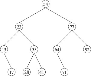
The hierarchical nature of this structure allows us to do something like
a binary search to find a key. Suppose, for example, that we are looking
for 41 in the above tree. We first compare 41 with the key in the root.
Because 41 < 54, we can safely ignore the right child, as all
keys there must be greater than 54. We therefore compare 41 to the key
in the root of the left child. Because 41 > 23, we look in the
right child, and compare 41 to 35. Because 41 > 35, we look in
the right child, where we find the key we are looking for.
Note the similarity of the search described above to a binary search. It
isn’t exactly the same, because there is no guarantee that the root is
the middle element in the tree — in fact, it could be the first or the
last. In many applications, however, when we build a binary search tree
as we will describe below, the root of the tree tends to be roughly the
middle element. When this is the case, looking up a key is very
efficient. Later
, we will
show how we can build and maintain a binary search tree so that this is
always the case.
It isn’t hard to implement the search strategy outlined above using a
loop. However, in order to reinforce the concept of recursion as a tree
processing technique, let’s consider how we would implement the search
using recursion. The algorithm breaks into four cases:
- The tree is empty. In this case, the element we are looking for is
not present.
- The key we are looking for is at the root - we have found what we
are looking for.
- The key we are looking for is less than the key at the root. We then
need to look for the given key in the left child. Because this is a
smaller instance of our original problem, we can solve it using a
recursive call.
- The key we are looking for is greater than the key at the root. We
then look in the right child using a recursive call.
Warning
It is important to handle the case of an empty tree first, as the other
cases don’t make sense if the tree is empty. In fact, if we are using
null to represent an empty binary search tree (as is fairly common),
we will get a compiler warning if we don’t do this, and ultimately a NullReferenceException if we try to access the key
at an empty root.
If we need to compare
elements using a
CompareTo
method, it would be more efficient to structure the code so that this
method is only called once; e.g.,
- If the tree is empty . . . .
- Otherwise:
- Get the result of the comparison.
- If the result is 0 . . . .
- Otherwise, if the result is negative . . . .
- Otherwise . . . .
This method would need to take two parameters — the key we are looking
for and the tree we are looking in. This second parameter will actually
be a reference to a node, which will either be the root of the tree or
null if the tree is empty. Because this method requires a parameter
that is not provided to the TryGetValue method, this method would be
a private method that the TryGetValue method can call. This
private method would then return the node containing the key, or
null if this key was not found. The TryGetValue method can be
implemented easily using this private method.
We also need to be able to implement the Add method. Let’s first
consider how to do this assuming we are representing our binary search
tree with immutable nodes. The first thing to observe is that because we
can’t modify an immutable node, we will need to build a binary search
tree containing the nodes in the current tree, plus a new node
containing the new key and value. In order to accomplish this, we will
describe a private recursive method that returns the result of
adding a given key and value to a given binary search tree. The Add
method will then need to call this private method and save the
resulting tree.
We therefore want to design a private method that will take three
parameters:
- a binary search tree (i.e., reference to a node);
- the key we want to add; and
- the value we want to add.
It will return the binary search tree that results from adding the given
key and value to the given tree.
This method again has four cases:
- The tree is empty. In this case, we need to construct a node
containing the given key and value and two empty children, and
return this node as the resulting tree.
- The root of the tree contains a key equal to the given key. In this
case, we can’t add the item - we need to throw an exception.
- The given key is less than the key at the root. We can then use a
recursive call to add the given key and value to the left child. The
tree returned by the recursive call needs to be the left child of
the result to be returned by the method. We therefore construct a
new node containing the data and right child from the given tree,
but having the result of the recursive call as its left child. We
return this new node.
- The given key is greater than the key at the root. We use a
recursive call to add it to the right child, and construct a new
node with the result of the recursive call as its right child. We
return this new node.
Note that the above algorithm only adds the given data item when it
reaches an empty tree. Not only is this the most straightforward way to
add items, but it also tends to keep paths in the tree short, as each
insertion is only lengthening one path. This
page
contains an
application that will
show the result of adding a key at a time to a binary search tree.
Warning
The
keys in this application are treated as strings; hence, you can use
numbers if you want, but they will be compared as strings (e.g.,
“10” < “5” because ‘1’ < ‘5’). For this reason, it is
usually better to use either letters, words, or integers that all have
the same number of digits.
The above algorithm can be implemented in the same way if mutable binary
tree nodes are used; however, we can improve its performance a bit by
avoiding the construction of new nodes when recursive calls are made.
Instead, we can change the child to refer to the tree returned. If we
make this optimization, the tree we return will be the same one that we
were given in the cases that make recursive calls. However, we still
need to construct a new node in the case in which the tree is empty. For
this reason, it is still necessary to return the resulting tree, and we
need to make sure that the Add method always uses the returned tree.
Removing from a Binary Search Tree
Removing from a Binary Search Tree
Before we can discuss how to remove an element from a binary search
tree, we must first define exactly how we want the method to behave.
Consider first the case in which the tree is built from immutable nodes.
We are given a key and a binary search tree, and we want to return the
result of removing the element having the given key. However, we need to
decide what we will do if there is no element having the given key. This
does not seem to be exceptional behavior, as we may have no way of
knowing in advance whether the key is in the tree (unless we waste time
looking for it). Still, we might want to know whether the key was found.
We therefore need two pieces of information from this method - the
resulting tree and a bool indicating whether the key was found. In
order to accommodate this second piece of information, we make the
bool an out parameter
.
We can again break the problem into cases and use recursion, as we did
for adding an element
. However, removing an element is complicated by the fact that its node
might have two nonempty children. For example, suppose we want to remove
the element whose key is 54 in the following binary search tree:

In order to preserve the correct ordering of the keys, we should replace
54 with either the next-smaller key (i.e., 41) or the next-larger key
(i.e., 64). By convention, we will replace it with the next-larger key,
which is the smallest key in its right child. We therefore have a
sub-problem to solve - removing the element with the smallest key from a
nonempty binary search tree. We will tackle this problem first.
Because we will not need to remove the smallest key from an empty tree,
we don’t need to worry about whether the removal was successful - a
nonempty binary search tree always has a smallest key. However, we still
need two pieces of information from this method:
- the element removed (so that we can use it to replace the element to
be removed in the original problem); and
- the resulting tree (so that we can use it as the new right child in
solving the original problem).
We will therefore use an out parameter for the element removed, and
return the resulting tree.
Because we don’t need to worry about empty trees, and because the
smallest key in a binary search tree is never larger than the key at the
root, we only have two cases:
- The left child is empty. In this case, there are no keys smaller
than the key at the root; i.e., the key at the root is the smallest.
We therefore assign the data at the root to the out parameter,
and return the right child, which is the result of removing the
root.
- The left child is nonempty. In this case, there is a key smaller
than the key at the root; furthermore, it must be in the left child.
We therefore use a recursive call on the left child to obtain the
result of removing the element with the smallest key from that child. We
can pass as the out parameter to this recursive call the out
parameter that we were given - the recursive call will assign to it
the element removed. Because our nodes are immutable, we then need to construct a new node whose data
and right child are the same as in the given tree, but whose left
child is the tree returned by the recursive call. We return this
node.
Having this sub-problem solved, we can now return to the original
problem. We again have four cases, but one of these cases breaks into
three sub-cases:
- The tree is empty. In this case the key we are looking for is not
present, so we set the out parameter to false and return an
empty tree.
- The key we are looking for is at the root. In this case, we can set
the out parameter to true, but in order to remove the
element, we have three sub-cases:
- The left child is empty. We can then return the right child (the
result of removing the root).
- The right child is empty. We can then return the left child.
- Both children are nonempty. We must then obtain the result of
removing the smallest key from the right child. We then
construct a new node whose data is the element removed from the
right child, the left child is the left child of the given tree,
and the right child is the result of removing the smallest key
from that child. We return this node.
- The key we are looking for is less than the key at the root. We then
obtain the result of removing this key from the left child using a
recursive call. We can pass as the out parameter to this
recursive call the out parameter we were given and let the
recursive call set its value. We then construct a new node whose
data and right child are the same as in the given tree, but whose
left child is the tree returned by the recursive call. We return
this node.
- The key we are looking for is greater than the key at the root. This
case is symmetric to the above case.
As we did with adding elements, we can optimize the methods described
above for mutable nodes by modifying the contents of a node rather than
constructing new nodes.
Inorder Traversal
Inorder Traversal
When we store keys and values in an ordered dictionary, we typically
want to be able to process the keys in increasing order. The
“processing” that we do may be any of a number of things - for example,
writing the keys and values to a file or adding them to the end of a
list. Whatever processing we want to do, we want to do it increasing
order of keys.
If we are implementing the dictionary using a binary search tree, this
may at first seem to be a rather daunting task. Consider traversing the
keys in the following binary search tree in increasing order:

Processing these keys in order involves frequent jumps in the tree, such
as from 17 to 23 and from 41 to 54. It may not be immediately obvious
how to proceed. However, if we just think about it with the purpose of
writing a recursive method, it actually becomes rather straightforward.
As with most tree-processing algorithms, if the given tree is nonempty,
we start at the root (if it is empty, there are no nodes to process).
However, the root isn’t necessarily the first node that we want to
process, as there may be keys that are smaller than the one at the root.
These key are all in the left child. We therefore want to process first
all the nodes in the left child, in increasing order of their keys. This
is a smaller instance of our original problem - a recursive call on the
left child solves it. At this point all of the keys less than the one at
the root have been processed. We therefore process the root next
(whatever the “processing” might be). This just leaves the nodes in the
right child, which we want to process in increasing order of their keys.
Again, a recursive call takes care of this, and we are finished.
The entire algorithm is therefore as follows:
- If the given tree is nonempty:
- Do a recursive call on the left child to process all the nodes
in it.
- Process the root.
- Do a recursive call on the right child to process all the nodes
in it.
This algorithm is known as an inorder traversal because it processes
the root between the processing of the two children. Unlike preorder
traversal
, this
algorithm only makes sense for binary trees, as there must be exactly
two children in order for “between” to make sense.
AVL Trees
AVL Trees
Up to this point, we haven’t addressed the performance of binary search
trees. In considering this performance, let’s assume that the time
needed to compare two keys is bounded by some fixed constant. The main
reason we do this is that this cost doesn’t depend on the number of keys
in the tree; however, it may depend on the sizes of the keys, as, for
example, if keys are strings. However, we will ignore this
complication for the purpose of this discussion.
Each of the methods we have described for finding a key, adding a key
and a value, or removing a key and its associated value, follows a
single path in the given tree. As a result, the time needed for each of
these methods is at worst proportional to the height of the tree,
where the height is defined to be the length of the longest path from
the root to any node. (Thus, the height of a one-node tree is
$ 0 $, because
no steps are needed to get from the root to the only node - the root
itself — and the height of a two-node tree is always
$ 1 $.) In other words,
we say that the worst-case running time of each of these methods is in
$ O(h) $, where
$ h $ is the height of the tree.
Depending on the shape of the tree,
$ O(h) $ running time might be very
good. For example, it is possible to show that if keys are randomly
taken from a uniform distribution and successively added to an initially
empty binary search tree, the expected height is in
$ O(\log n) $,
where
$ n $ is the number of nodes. In this case, we would expect
logarithmic performance for lookups, insertions, and deletions. In fact,
there are many applications in which the height of a binary search tree
remains fairly small in comparison to the number of nodes.
On the other hand, such a shape is by no means guaranteed. For example,
suppose a binary search tree were built by adding the int keys 1
through
$ n $ in increasing order. Then 1 would go at the root, and 2
would be its right child. Each successive key would then be larger than
any key currently in the tree, and hence would be added as the right
child of the last node on the path going to the right. As a result, the
tree would have the following shape:
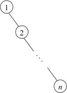
The height of this tree is
$ n - 1 $; consequently, lookups will
take time linear in
$ n $, the number of elements, in the worst case. This
performance is comparable with that of a linked list. In order to
guaranteed good performance, we need a way to ensure that the height of
a binary search tree does not grow too quickly.
One way to accomplish this is to require that each node always has
children that differ in height by at most
$ 1 $. In order for this
restriction to make sense, we need to extend the definition of the
height of a tree to apply to an empty tree. Because the height of a
one-node tree is
$ 0 $, we will define the height of an empty tree to be
$ -1 $.
We call this restricted form of a binary search tree an AVL tree
(“AVL” stands for the names of the inventors, Adelson-Velskii and
Landis).
This repository
contains a Java application that displays an AVL tree of a given
height using as few nodes as possible. For example, the following screen
capture shows an AVL tree of height
$ 7 $ having a minimum number of nodes:
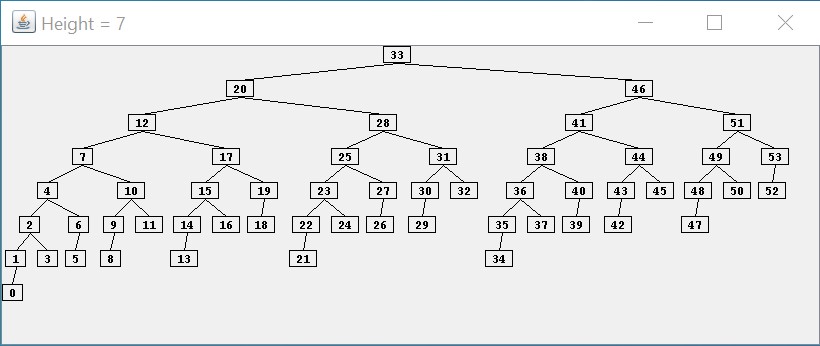
As the above picture illustrates, a minimum of
$ 54 $ nodes are required for
an AVL tree to reach a height of
$ 7 $. In general, it can be shown that the
height of an AVL tree is at worst proportional to
$ \log n $, where
$ n $
is the number of nodes in the tree. Thus, if we can maintain the shape
of an AVL tree efficiently, we should have efficient lookups and
updates.
Regarding the AVL tree shown above, notice that the tree is not as
well-balanced as it could be. For example,
$ 0 $ is at depth
$ 7 $, whereas
$ 52 $,
which also has two empty children, is only at depth
$ 4 $. Furthermore, it
is possible to arrange
$ 54 $ nodes into a binary tree with height as small
as
$ 5 $. However, maintaining a more-balanced structure would likely
require more work, and as a result, the overall performance might not be
as good. As we will show in what follows, the balance criterion for an
AVL tree can be maintained without a great deal of overhead.
The first thing we should consider is how we can efficiently determine
the height of a binary tree. We don’t want to have to explore the entire
tree to find the longest path from the root — this would be way too
expensive. Instead, we store the height of a tree
in its root. If our nodes are mutable, we should use a
public property with both get and set accessors for this purpose. However,
such a setup places the burden of maintaining the heights on the user of
the binary tree node class. Using immutable nodes allows a much cleaner
(albeit slightly less efficient) solution. In what follows, we will show
how to modify the definition of an immutable binary tree node so that
whenever a binary tree is created from such nodes, the resulting tree is
guaranteed to satisfy the AVL tree balance criterion. As a result, user
code will be able to form AVL trees as if they were ordinary binary
search trees.
In order to allow convenient and efficient access to the height, even
for empty trees, we can store the height of a tree in a private field in its root, and provide a static method to take a nullable binary
tree node as its only parameter and return its height. Making this
method static will allow us to handle empty (i.e., null) trees.
If the tree is empty, this method will return
$ -1 $; otherwise, it will
return the height stored in the tree. This method can be public.
We then can modify the constructor so that it initializes the height
field. Using the above method, it can find the heights of each child,
and add
$ 1 $ to the maximum of these values. This is the height of the node
being constructed. It can initialize the height field to this value, and
because the nodes are immutable, this field will store the correct
height from that point on.
Now that we have a way to find the height of a tree efficiently, we can
focus on how we maintain the balance property. Whenever an insertion or
deletion would cause the balance property to be violated for a
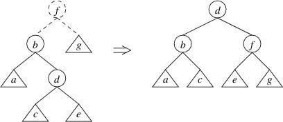
particular node, we perform a rotation at that node. Suppose, for
example, that we have inserted an element into a node’s left child, and
that this operation causes the height of the new left child to be
$ 2 $
greater than the height of the right child (note that this same scenario
could have occurred if we had removed an element from the right child).
We can then rotate the tree using a single rotate right:
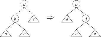
The tree on the left above represents the tree whose left child has a
height
$ 2 $ greater than its right child. The root and the lines to its
children are drawn using dashes to indicate that the root node has not
yet been constructed — we have at this point simply built a new left
child, and the tree on the left shows the tree that would be formed if
we were building an ordinary binary search tree. The circles in the
picture indicate individual nodes, and the triangles indicate arbitrary
trees (which may be empty). Note that the because the left child has a
height
$ 2 $ greater than the right child, we know that the left child
cannot be empty; hence, we can safely depict it as a node with two
children. The labels are chosen to indicate the order of the elements —
e.g., as “a”
$ \lt $ “b”, every key in tree a is less than the key in
node b. The tree on the right shows the tree that would be built by
performing this rotation. Note that the rotation preserves the order of
the keys.
Suppose the name of our class implementing a binary tree node is
BinaryTreeNode<T>, and suppose it has the following properties:
- Data: gets the data stored in the node.
- LeftChild: gets the left child of the node.
- RightChild: gets the right child of the node.
Then the following code can be used to perform a single rotate right:
/// <summary>
/// Builds the result of performing a single rotate right on the binary tree
/// described by the given root, left child, and right child.
/// </summary>
/// <param name="root">The data stored in the root of the original tree.</param>
/// <param name="left">The left child of the root of the original tree.</param>
/// <param name="right">The right child of the root of the original tree.</param>
/// <returns>The result of performing a single rotate right on the tree described
/// by the parameters.</returns>
private static BinaryTreeNode<T> SingleRotateRight(T root,
    BinaryTreeNode<T> left, BinaryTreeNode<T>? right)
{
    BinaryTreeNode<T> newRight = new(root, left.RightChild, right);
    return new BinaryTreeNode<T>(left.Data, left.LeftChild, newRight);
}
Relating this code to the tree on the left in the picture above, the
parameter root refers to d, the parameter left refers to the tree
rooted at node b, and the parameter right refers to the (possibly empty) tree e. The
code first constructs the right child of the tree on the right and
places it in the variable newRight. It then constructs the entire tree
on the right and returns it.
Warning
Don’t try to write the code for doing rotations without looking at pictures of the rotations.
Now that we have seen what a single rotate right does and how to code
it, we need to consider whether it fixes the problem. Recall that we
were assuming that the given left child (i.e., the tree rooted at b in
the tree on the left above) has a height
$ 2 $ greater than the given right
child (i.e., the tree e in the tree on the left above). Let’s suppose
the tree e has height
$ h $. Then the tree rooted at b has height
$ h + 2 $. By the definition of the height of a tree, either a
or c (or both) must have height
$ h + 1 $. Assuming that every
tree we’ve built so far is an AVL tree, the children of b must differ
in height by at most
$ 1 $; hence, a and c must both have a height of at
least
$ h $ and at most
$ h + 1 $.
Given these heights, let’s examine the tree on the right. We have
assumed that every tree we’ve built up to this point is an AVL tree, so
we don’t need to worry about any balances within a, c, or e.
Because c has either height
$ h $ or height
$ h + 1 $ and e has
height
$ h $, the tree rooted at d satisfies the balance criterion.
However, if c has height
$ h + 1 $ and a has height
$ h $, then
the tree rooted at d has height
$ h + 2 $, and the balance
criterion is not satisfied. On the other hand, if a has height
$ h + 1 $, the tree rooted at d will have a height of either
$ h + 1 $ or
$ h + 2 $, depending on the height of c. In these
cases, the balance criterion is satisfied.
We therefore conclude that a single rotate right will restore the
balance if:
- The height of the original left child (i.e., the tree rooted at b
in the above figure) is
$ 2 $ greater than the height of the original
right child (tree e in the above figure); and
- The height of the left child of the original left child (tree a in
the above figure) is greater than the height of the original right
child (tree e).
For the case in which the height of the left child of the original left
child (tree a) is not greater than the height of the original right
child (tree e), we will need to use a different kind of rotation.
Before we consider the other kind of rotation, we can observe that if an
insertion or deletion leaves the right child with a height
$ 2 $ greater
than the left child and the right child of the right child with a height
greater than the left child, the mirror image of a single rotate right
will restore the balance. This rotation is called a single rotate
left:
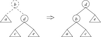
Returning to the case in which the left child has a height
$ 2 $ greater
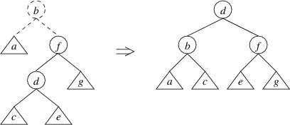
than the right child, but the left child of the left child has a height
no greater than the right child, we can in this case do a double rotate
right:
Note that we have drawn the trees a bit differently by showing more
detail. Let’s now show that this rotation restores the balance in this
case. Suppose that in the tree on the left, g has height
$ h $. Then the
tree rooted at b has height
$ h + 2 $. Because the height of a
is no greater than the height of g, assuming all trees we have built
so far are AVL trees, a must have height
$ h $, and the tree rooted at
d must have height
$ h + 1 $ (thus, it makes sense to draw it as
having a root node). This means that c and e both must have heights
of either
$ h $ or
$ h - 1 $. It is now not hard to verify that the
balance criterion is satisfied at b, f, and d in the tree on the
right.
The only remaining case is the mirror image of the above — i.e., that
the right child has height
$ 2 $ greater than the left child, but the height
of the right child of the right child is no greater than the height of
the left child. In this case, a double rotate left can be applied:
We have shown how to restore the balance whenever the balance criterion
is violated. Now we just need to put it all together in a public
static method that will replace the constructor as far as user code is
concerned. In order to prevent the user from calling the constructor
directly, we also need to make the constructor private. We want this
static method to take the same parameters as the constructor:
- The data item that can be stored at the root, provided no rotation
is required.
- The tree that can be used as the left child if no rotation is
required.
- The tree that can be used as the right child if no rotation is
required.
The purpose of this method is to build a tree including all the given
nodes, with the given data item following all nodes in the left child
and preceding all nodes in the right child, but satisfying the AVL tree
balance criterion. Because this method will be the only way for user
code to build a tree, we can assume that both of the given trees satisfy
the AVL balance criterion. Suppose that the name of the static
method to get the height of a tree is Height, and that the names of
the methods to do the remaining rotations are SingleRotateLeft,
DoubleRotateRight, and DoubleRotateLeft, respectively. Further
suppose that the parameter lists for each of these last three methods
are the same as for SingleRotateRight above, except that for the left rotations, left is nullable, not right. The following method
can then be used to build AVL trees:
/// <summary>
/// Constructs an AVL Tree from the given data element and trees. The heights of
/// the trees must differ by at most two. The tree built will have the same
/// inorder traversal order as if the data were at the root, left were the left
/// child, and right were the right child.
/// </summary>
/// <param name="data">A data item to be stored in the tree.</param>
/// <param name="left">An AVL Tree containing elements less than data.</param>
/// <param name="right">An AVL Tree containing elements greater than data.
/// </param>
/// <returns>The AVL Tree constructed.</returns>
public static BinaryTreeNode<T> GetAvlTree(T data, BinaryTreeNode<T>? left,
    BinaryTreeNode<T>? right)
{
    int diff = Height(left) - Height(right);
    if (Math.Abs(diff) > 2)
    {
        throw new ArgumentException();
    }
    else if (diff == 2)
    {
        // If the heights differ by 2, left's height is at least 1; hence, it isn't null.
        if (Height(left!.LeftChild) > Height(right))
        {
            return SingleRotateRight(data, left, right);
        }
        else
        {
            // If the heights differ by 2, but left.LeftChild's height is no more than
            // right's height, then left.RightChild's height must be greater than right's
            // height; hence, left.RightChild isn't null.
            return DoubleRotateRight(data, left, right);
        }
    }
    else if (diff == -2)
    {
        // If the heights differ by -2, right's height is at least 1; hence, it isn't null.
        if (Height(right!.RightChild) > Height(left))
        {
            return SingleRotateLeft(data, left, right);
        }
        else
        {
            // If the heights differ by -1, but right.RightChild's height is no more than
            // left's height, then right.LeftChild's height must be greater than right's
            // height; hence right.LeftChild isn't null.
            return DoubleRotateLeft(data, left, right);
        }
    }
    else
    {
        return new BinaryTreeNode<T>(data, left, right);
    }
}
In order to build and maintain an AVL tree, user code simply needs to
call the above wherever it would have invoked the
BinaryTreeNode<T> constructor in building and maintaining an
ordinary binary search tree. The extra overhead is fairly minimal — each
time a new node is constructed, we need to check a few heights (which
are stored in fields), and if a rotation is needed, construct one or two
extra nodes. As a result, because the height of an AVL tree is
guaranteed to be logarithmic in the number of nodes, the worst-case
running times of both lookups and updates are in
$ O(\log n) $, where
$ n $ is the number of nodes in the tree.
Subsections of Tries
Introduction to Tries
Introduction to Tries
A trie is a nonempty tree storing a set of words in the following way:
- Each child of a node is labeled with a character.
- Each node contains a boolean indicating whether the labels in the
path from the root to that node form a word in the set.
The word, “trie”, is taken from the middle of the word, “retrieval”, but
to avoid confusion, it is pronounced like “try” instead of like “tree”.
Suppose, for example, that we want to store the following words:
- ape
- apple
- cable
- car
- cart
- cat
- cattle
- curl
- far
- farm
A trie storing these words (where we denote a value of true for the
boolean with a *) is as follows:
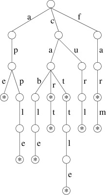
Thus, for example, if we follow the path from the root through the
labels ‘c’, ‘a’, and ‘r’, we reach a node with a true boolean value
(shown by the * in the above picture); hence, “car” is in this set of
words. However, if we follow the path through the labels ‘c’, ‘u’, and
‘r’, the node we reach has a false boolean; hence, “cur” is not in
this set. Likewise, if we follow the path through ‘a’, we reach a node
from which there is no child labeled ‘c’; hence, “ace” is not in this
set.
Note that each subtree of a trie is also a trie, although the “words” it
stores may begin to look a little strange. For example if we follow the
path through ‘c’ and ‘a’ in the above figure, we reach a trie that
contains the following “words”:
- “ble”
- “r”
- “rt”
- “t”
- “ttle”
These are actually the completions of the original words that begin
with the prefix “ca”. Note that if, in this subtree, we take the path
through ’t’, we reach a trie containing the following completions:
- "" [i.e., the empty string]
- “tle”
In particular, the empty string is a word in this trie. This motivates
an alternative definition of the boolean stored in each node: it
indicates whether the empty string is stored in the trie rooted at this
node. This definition may be somewhat preferable to the one given above,
as it does not depend on any context, but instead focuses entirely on
the trie rooted at that particular node.
One of the main advantages of a trie over an AVL
tree
is the speed with
which we can look up words. Assuming we can quickly find the child with
a given label, the time we need to look up a word is proportional to the
length of the word, no matter how many words are in the trie. Note that
in looking up a word that is present in an AVL tree, we will at least
need to compare the given word with its occurrence in the tree, in
addition to any other comparisons done during the search. The time it
takes to do this one comparison is proportional to the length of the
word, as we need to verify each character (we actually ignored the cost
of such comparisons when we analyzed the performance of AVL trees).
Consequently, we can expect a significant performance improvement by
using a trie if our set of words is large.
Let’s now consider how we can implement a trie. There are various ways
that this can be done, but we’ll consider a fairly straightforward
approach in this section (we’ll improve the implementation in the next
section
). We
will assume that the words we are storing are comprised of only the 26
lower-case English letters. In this implementation, a single node will
contain the following private fields:
- A bool storing whether the empty string is contained in the trie
rooted at this node (or equivalently, whether this node ends a word
in the entire trie).
- A 26-element array of nullable tries storing the children, where element 0
stores the child labeled ‘a’, element 1 stores the child labeled
‘b’, etc. If there is no child with some label, the corresponding
array element is null.
For maintainability, we should use private constants to store the above array’s size (i.e., 26) and the first letter of the alphabet (i.e., ‘a’). Note that in this implementation, other than this last constant, no chars or strings are
actually stored. We can see if a node has a child labeled by a given
char by finding the difference between that char and and the first letter of the alphabet, and
using that difference as the array index. For example, suppose the array
field is named _children, the constant giving the first letter of the alphabet is _alphabetStart, and label is a char variable
containing a lower-case letter. Because char is technically a
numeric type, we can perform arithmetic with chars; thus, we can
obtain the child labeled by label by retrieving
_children[label - _alphabetStart]. More specifically, if _alphabetStart is ‘a’ and label
contains ’d’, then the difference, label - _alphabetStart, will be 3; hence,
the child with label ’d’ will be stored at index 3. We have therefore
achieved our goal of providing quick access to a child with a given
label.
Let’s now consider how to implement a lookup. We can define a public
method for this purpose within the class implementing a trie node:
public bool Contains(string s)
{

    . . .

}
Note
This method does not need a trie node as a parameter because
the method will belong to a trie node. Thus, the method will be able to
access the node as
this
, and may
access its private fields directly by their names.
The method
consists of five cases:
s is null. Note that even though s is not defined to be nullable, because the method is public, user code could still pass a null value. In this case, we should throw an ArgumentNullException, provides more information than does a NullReferenceException.s is the empty string. In this case the bool stored in
this node indicates whether it is a word in this trie; hence, we can
simply return this bool.- The first character of
s is not a lower-case English letter (i.e.,
it is less than ‘a’ or greater than ‘z’). The constants defined for this class should be used in making this determination. In this case, s can’t be stored
in this trie; hence, we can return false.
- The child labeled with the first character of
s (obtained as
described above) is missing (i.e., is null). Then s isn’t
stored in this trie. Again, we return false.
- The child labeled with the first character of
s is present (i.e.,
non-null). In this case, we need to determine whether the
substring following the first character of s is in the trie rooted
at the child we retrieved. This can be found using a recursive call
to this method within the child trie node. We return the result of
this recursive call.
In order to be able to look up words, we need to be able to build a trie
to look in. We therefore need to be able to add words to a trie. It’s
not practical to make a trie node immutable, as there is too much
information that would need to be copied if we need to replace a node
with a new one (we would need to construct a new node for each letter of
each word we added). We therefore should provide a public method
within the trie node class for the purpose of adding a word to the trie
rooted at this node:
public void Add(string s)
{

    . . .

}
This time there are four cases:
s is null. This case should be handled as in the Contains method above.s is the empty string. Then we can record this word by setting
the bool in this node to true.- The first character of
s is not a lower-case English letter. Then
we can’t add the word. In this case, we’ll need to throw an
exception.
- The first character is a lower-case English letter. In this case, we
need to add the substring following the first character of
s to
the child labeled with the first letter. We do this as follows:
- We first need to make sure that the child labeled with the first letter of
s is non-null. Thus, if this child is null, we construct a new trie node and place
it in the array location for this child.
- We can now
add the substring following the first letter of
s to this child by
making a recursive call.
Multiple Implementations of Children
Multiple Implementations of Children
The trie implementation given in the previous
section
offers very
efficient lookups - a word of length
$ m $ can be looked up in
$ O(m) $
time, no matter how many words are in the trie. However, it wastes a
large amount of space. In a typical trie, a majority of the nodes will
have no more than one child; however, each node contains a 26-element
array to store its children. Furthermore, each of these arrays is
automatically initialized so that all its elements are null. This
initialization takes time. Hence, building a trie may be rather
inefficient as well.
We can implement a trie more efficiently if we can customize the
implementation of a node based on the number of children it has. Because
most of the nodes in a trie can be expected to have either no children
or only one child, we can define alternate implementations for these
special cases:
- For a node with no children, there is no need to represent any
children - we only need the bool indicating whether the trie
rooted at this node contains the empty string.
- For a node with exactly one child, we maintain a single reference to
that one child. If we do this, however, we won’t be able to infer
the child’s label from where we store the child; hence, we also need
to have a char giving the child’s label. We also need the
bool indicating whether the trie rooted at this node contains
the empty string.
For all other nodes, we can use an implementation similar to the one
outlined in the previous
section
. We will still
waste some space with the nodes having more than one child but fewer
than 26; however, the amount of space wasted will now be much less.
Furthermore, in each of these three implementations, we can quickly
access the child with a given label (or determine that there is no such
child).
Conceptually, this sounds great, but we run into some obstacles as soon
as we try to implement this approach. Because we are implementing nodes
in three different ways, we need to define three different classes. Each
of these classes defines a different type. So how do we build a trie
from three different types of nodes? In particular, how do we define the
type of a child when that child may be any of three different types?
The answer is to use a C# construct called an interface. An interface
facilitates abstraction - hiding lower-level details in order to focus
on higher-level details. At a high level (i.e., ignoring the specific
implementations), these three different classes appear to be the same:
they are all used to implement tries of words made up of lower-case
English letters. More specifically, we want to be able to add a
string to any of these classes, as well as to determine whether they
contain a given string. An interface allows us to define a type that
has this functionality, and to define various sub-types that have
different implementations, but still have this functionality.
A simple example of an interface is
IComparable<T>
.
Recall from the section, “Implementing a Dictionary with a Linked
List”
,
that we can constrain the keys in a dictionary implementation to be of a
type that can be ordered by using a where clause on the class
statement, as follows:
public class Dictionary<TKey, TValue> where TKey : notnull, IComparable<TKey>
The source code for the IComparable<T>
interface
has been posted by Microsoft®. The essential part of this definition
is:
public interface IComparable<in T>
{
    int CompareTo(T? other);
}
(Don’t worry about the in keyword with the type parameter in the
first line.) This definition defines the type IComparable<T> as
having a method CompareTo that takes a parameter of the generic type
T? and returns an int. Note that there is no public or
private access modifier on the method definition. This is because
access modifiers are disallowed within interfaces — all definitions are
implicitly public. Note also that there is no actual definition of
the CompareTo method, but only a header followed by a semicolon.
Definitions of method bodies are also disallowed within interfaces — an
interface doesn’t define the behavior of a method, but only how it
should be used (i.e., its parameter list and return type). For this
reason, it is impossible to construct an instance of an interface
directly. Instead, one or more sub-types of the interface must be
defined, and these sub-types must provide definitions for the behavior
of CompareTo. As a result, because the Dictionary<TKey,
TValue> class restricts type TKey to be a sub-type of
IComparable<T>, its can use the CompareTo method of any
instance of type TKey.
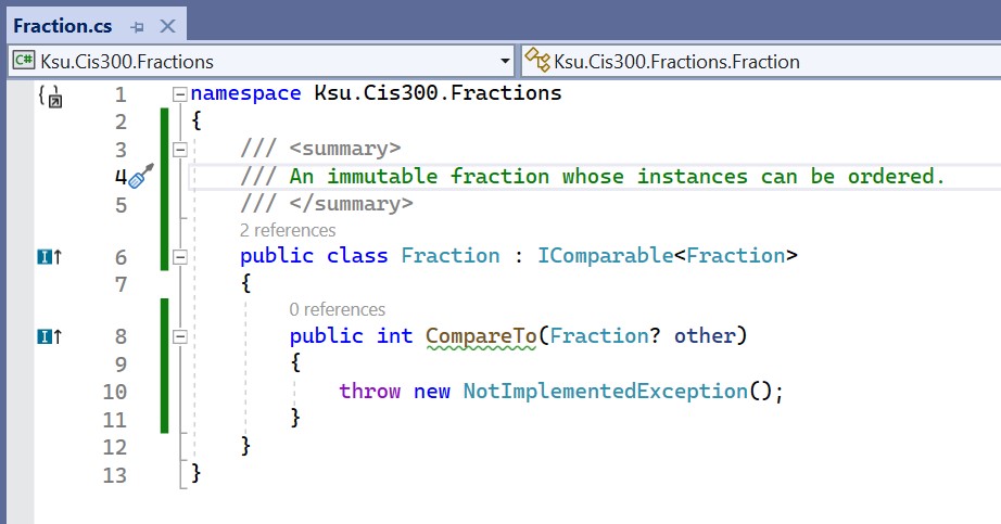
Now suppose that we want to define a class Fraction and use it as a
key in our dictionary implementation. We would begin the class
definition within Visual Studio® as follows:
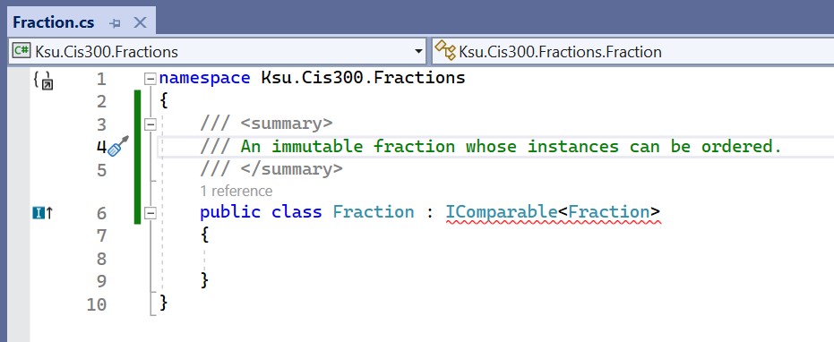
At the end of the first line of the class definition, : IComparable<Fraction> indicates that the class being defined is a
subtype of IComparable<Fraction>. In general, we can list one or
more interface names after the colon, separating these names with
commas. Each name that we list requires that all of the methods,
properties, and indexers
from that interface must be fully defined within this class. If we hover
the mouse over the word, IComparable<Fraction>, a drop-down menu
appears. By selecting “Implement interface” from this menu, all of the
required members of the interface are provided for us:
Note
In order to implement a method specified in an interface, we
must define it as public.
We now just need to replace the throw
with the proper code for the CompareTo method and fill in any other
class members that we need; for example:
namespace Ksu.Cis300.Fractions
{
    /// <summary>
    /// An immutable fraction whose instances can be ordered.
    /// </summary>
    public class Fraction : IComparable<Fraction>
    {
        /// <summary>
        /// Gets the numerator.
        /// </summary>
        public int Numerator { get; }

        /// <summary>
        /// Gets the denominator.
        /// </summary>
        public int Denominator { get; }

        /// <summary>
        /// Constructs a new fraction with the given numerator and denominator.
        /// </summary>
        /// <param name="numerator">The numerator.</param>
        /// <param name="denominator">The denominator.</param>
        public Fraction(int numerator, int denominator)
        {
            if (denominator <= 0)
            {
                throw new ArgumentException();
            }
            Numerator = numerator;
            Denominator = denominator;
        }

        /// <summary>
        /// Compares this fraction with the given fraction.
        /// </summary>
        /// <param name="other">The fraction to compare to.</param>
        /// <returns>A negative value if this fraction is less
        /// than other, 0 if they are equal, or a positive value if this
        /// fraction is greater than other or if other is null.</returns>
        public int CompareTo(Fraction? other)
        {
            if (other == null)
            {
                return 1;
            }
            long prod1 = (long)Numerator * other.Denominator;
            long prod2 = (long)other.Numerator * Denominator;
            return prod1.CompareTo(prod2);
        }

        // Other class members
    }
}
Note
The CompareTo method above is not recursive. The
CompareTo method that it calls is a member of the long
structure, not the Fraction class.
As we suggested above, interfaces can also include properties. For
example,
ICollection<T>
is a generic interface implemented by both arrays and the class
List<T>
.
This interface contains the following member (among others):
This member specifies that every subclass must contain a property called
Count with a getter. At first, it would appear that an array does
not have such a property, as we cannot write something like:
int[] a = new int[10];
int k = a.Count;  // This gives a syntax error.
In fact, an array does contain a
Count property, but this property is available only when the array
is treated as an ICollection<T> (or an
IList<T>
,
which is an interface that is a subtype of ICollection<T>, and is
also implemented by arrays). For example, we can write:
int[] a = new int[10];
ICollection<int> col = a;
int k = col.Count;
or
int[] a = new int[10];
int k = ((ICollection<int>)a).Count;
This behavior occurs because an array explicitly implements the
Count property. We can do this as follows:
public class ExplicitImplementationExample<T> : ICollection<T>
{
    int ICollection<T>.Count
    {
        get
        {
            // Code to return the proper value
        }
    }

    // Other class members
}
Thus, if we create an instance of
ExplicitImplementationExample<T>, we cannot access its Count
property unless we either store it in a variable of type
ICollection<T> or cast it to this type. Note that whereas the
public access modifier is required when implementing an interface
member, neither the public nor the private access modifier is
allowed when explicitly implementing an interface member.
We can also include
indexers
within
interfaces. For example, the IList<T> interface is defined as
follows:
public interface IList<T> : ICollection<T>
{
    T this[int index] { get; set; }

    int IndexOf(T item);

    void Insert(int index, T item);

    void RemoveAt(int index);
}
The : ICollection<T> at the end of the first line specifies that
IList<T> is a subtype of ICollection<T>; thus, the interface
includes all members of ICollection<T>, plus the ones listed. The
first member listed above specifies an indexer with a get accessor and a
set accessor.
Now that we have seen a little of what interfaces are all about, let’s
see how we can use them to provide three different implementations of
trie nodes. We first need to define an interface, which we will call
ITrie, specifying the two public members of our previous
implementation of a trie
node
. We do, however,
need to make one change to the way the Add method is called. This
change is needed because when we add a string to a trie, we may need
to change the implementation of the root node. We can’t simply change
the type of an object - instead, we’ll need to construct a new instance
of the appropriate implementation. Hence, the Add method will need
to return the root of the resulting trie. Because this node may have any
of the three implementations, the return type of this method should be
ITrie. Also, because we will need the constants from our previous implementation in each of the implementations of ITrie, the code will be more maintainable if we include them once within this interface definition. Note that this will have the effect of making them public. The ITrie interface is therefore as follows:
/// <summary>
/// An interface for a trie.
/// </summary>
public interface ITrie
{
    /// <summary>
    /// The first character of the alphabet we use.
    /// </summary>
    const char AlphabetStart = 'a';

    /// <summary>
    /// The number of characters in the alphabet.
    /// </summary>
    const int AlphabetSize = 26;

    /// <summary>
    /// Determines whether this trie contains the given string.
    /// </summary>
    /// <param name="s">The string to look for.</param>
    /// <returns>Whether this trie contains s.</returns>
    bool Contains(string s);

    /// <summary>
    /// Adds the given string to this trie.
    /// </summary>
    /// <param name="s">The string to add.</param>
    /// <returns>The resulting trie.</returns>
    ITrie Add(string s);
}
We will then need to define three classes, each of which implements the
above interface. We will use the following names for these classes:
- TrieWithNoChildren will be used for nodes with no children.
- TrieWithOneChild will be used for nodes with exactly one child.
- TrieWithManyChildren will be used for all other nodes; this will
be the class described in the previous
section
with a few
modifications.
These three classes will be similar because they each will implement the
ITrie interface. This implies that they will each need a
Contains method and an Add method as specified by the interface
definition. However, the code for each of these methods will be
different, as will other aspects of the implementations.
Let’s first discuss how the TrieWithManyChildren class will differ from the class described in the previous
section
. First, its class statement will need to be modified to make the class implement the ITrie interface. This change will introduce a syntax error because the Add method in the ITrie interface has a return type of ITrie, rather than void. The return type of this method in the TrieWithManyChildren class will therefore need to be changed, and at the end this will need to be returned. Because the constants have been moved to the ITrie interface, their definitions will need to be removed from this class definition, and each occurrence will need to be prefixed by “ITrie.”. Throughout the class definition, the type of any trie should be made ITrie, except where a new trie is constructed in the Add method. Here, a new TrieWithNoChildren should be constructed.
Finally, a constructor needs to be defined for the TrieWithManyChildren class. This constructor will be used by the TrieWithOneChild class when it needs to add a new child. Because a TrieWithOneChild cannot have two children, a TrieWithManyChildren will need to be constructed instead. This constructor will need the following parameters:
- A string giving the string that the TrieWithOneChild class needs to add.
- A bool indicating whether the constructed node should contain the empty string.
- A char giving the label of the child stored by the TrieWithOneChild.
- An ITrie giving the one child of the TrieWithOneChild.
After doing some error checking to make sure the given string and ITrie are not null and that the given char is in the proper range, it will need to store the given bool in its bool field and store the given ITrie at the proper location of its array of children. Then, using its own Add method, it can add the given string.
Let’s now consider the TrieWithOneChild class. It will need three private fields:
- A bool indicating whether this node contains the empty string.
- A char giving the label of the only child.
- An ITrie giving the only child.
As with the TrieWithManyChildren class the TrieWithOneChild class needs a constructor to allow the TrieWithNoChildren class to be able to add a nonempty string. This constructor’s parameters will be a
string to be stored (i.e., the one being added) and a bool
indicating whether the empty string is also to be stored.
Furthermore, because the empty string can always be added to a
TrieWithNoChildren without constructing a new node, this constructor
should never be passed the empty string. The constructor can then
operate as follows:
- If the given string is null, throw an ArgumentNullException.
- If the given string is empty or begins with a character that is
not a lower-case English letter, throw an exception.
- Initialize the bool field with the given bool.
- Initialize the char field with the first character of the given
string.
- Initialize the ITrie field with the result of constructing a new
TrieWithNoChildren and adding to it the substring of the given
string following the first character.
The structure of the Contains method for the TrieWithOneChild class is similar to the TrieWithManyChildren class. Specifically, the
empty string needs to be handled first (after checking that the string isn’t null) and in exactly the same way,
as the empty string is represented in the same way in all three
implementations. Nonempty strings, however, are represented
differently, and hence need to be handled differently. For TrieWithOneChild, we need to check to
see if the first character of the given string matches the child’s
label. If so, we can recursively look for the remainder of the
string in that child. Otherwise, we should simply return false,
as this string is not in this trie.
The Add method for TrieWithOneChild will need five cases:
- A null string: This case can be handled in the same way as for TrieWithManyChildren.
- The empty string: This case can be handled in the same way as
for TrieWithManyChildren.
- A nonempty string whose first character is not a lower-case letter: An exception should be thrown.
- A nonempty string whose first character matches the child’s
label: The remainder of the string can be added to the child
using the child’s Add method. Because this method may return a
different node, we need to replace the child with the value this
method returns. We can then return this, as we didn’t need more
room for the given string.
- A nonempty string whose first character is a lower-case letter but does not match the
child’s label. In this case, we need to return a new
TrieWithManyChildren containing the given string and all of
the information already being stored.
The TrieWithNoChildren class is the simplest of the three, as we don’t need to worry about any children. The only private field it needs is a bool to indicate whether it stores the empty string. Its Contains method needs to handle null or empty strings in the same way as for the other two classes, but because a TrieWithNoChildren cannot contain a nonempty string, this method can simply return false when it is given a nonempty string.
The Add method for TrieWithNoChildren will need to handle a null or
empty string in the same way as the the other two classes. However,
this implementation cannot store a nonempty string. In this case, it
will need to construct and return a new TrieWithOneChild containing
the string to be added and the bool stored in this node.
Code that uses such a trie will need to refer to it as an ITrie
whenever possible. The only exception to this rule occurs when we are
constructing a new trie, as we cannot construct an instance of an
interface. Here, we want to construct the simplest implementation — a
TrieWithNoChildren. Otherwise, the only difference in usage as
compared to the implementation of the previous
section
is that the
Add method now returns the resulting trie, whose root may be a
different object; hence, we will need to be sure to replace the current
trie with whatever the Add method returns.
Traversing a Trie
Traversing a Trie
As with other kinds of trees, there are occasions where we need to
process all the elements stored in a trie in order. Here, the elements
are strings, which are not stored explicitly in the trie, but implicitly
based on the labels of various nodes. Thus, an individual node does not
contain a string; however, if its bool has a value of true,
then the path to that node describes a string stored in the trie. We can
therefore associate this string with this node. Note that this string is
a prefix of any string associated with any node in any of this node’s
children; hence, it is alphabetically less than any string found in any
of the children. Thus, in order to process each of the strings in
alphabetic order, we need to do a preorder
traversal
, which
processes the root before recursively processing the children.
In order to process the string associated with a node, we need to be
able to retrieve this string. Because we will have followed the path
describing this string in order to get to the node associated with it,
we can build this string on the way to the node and pass it as a
parameter to the preorder traversal of the trie rooted at this node.
Because we will be building this string a character at a time, to do
this efficiently we should use a
StringBuilder
instead of a string. Thus, the preorder traversal method for a trie
will take a StringBuilder parameter describing the path to that
trie, in addition to any other parameters needed to process the strings
associated with its nodes.
Before we present the algorithm itself, we need to address one more
important issue. We want the StringBuilder parameter to describe the
path to the node we are currently working on. Because we will need to do
a recursive call on each child, we will need to modify the
StringBuilder to reflect the path to that child. In order to be able
to do this, we will need to ensure that the recursive calls don’t change
the contents of the StringBuilder (or more precisely, that they undo
any changes that they make).
Because we are implementing a preorder traversal, the first thing we
will need to do is to process the root. This involves determining
whether the root is associated with a string contained in the trie, and
if so, processing that string. Determining whether the root is
associated with a contained string is done by checking the bool at
the root. If it is true, we can convert the StringBuilder
parameter to a string and process it by doing whatever processing
needs to be done for each string in our specific application.
Once we have processed the root, we need to recursively process each of
the children in alphabetic order of their labels. How we accomplish this
depends on how we are implementing the trie - we will assume the
implementation of the previous
section
. Because
this implementation uses three different classes depending on how many
children a node has, we will need to write three different versions of
the preorder traversal, one for each class. Specifically, after processing the root:
- For a TrieWithNoChildren, there is nothing more to do.
- Because a TrieWithOneChild has exactly one child, we need a
single recursive call on this child. Before we make this call, we
will need to append the child’s label to the StringBuilder.
Following the recursive call, we will need to remove the character
that we added by reducing its
Length
property by 1.
- We handle a TrieWithManyChildren in a similar way as a
TrieWithOneChild, only we will need to iterate through the
array of children and process each non-null child with a
recursive call. Note that for each of these children, its label will
need to be appended to the StringBuilder prior to the recursive
call and removed immediately after. We can obtain the label of a
child by adding the first letter of the alphabet to its array index and
casting
the result to a
char.
Tries in Word Games
Tries in Word Games
One application of tries is for implementing word games such as
Boggle® or Scrabble®. This section discusses how a trie can be
used to reduce dramatically the amount of time spent searching for words
in such games. We will focus specifically on Boggle, but the same
principles apply to other word games as well.
A Boggle game consists of either 16 or 25 dice with letters on their
faces, along with a tray containing a 4 x 4 or 5 x 5 grid
for holding these dice. The face of each die contains a single letter,
except that one face of one die contains “Qu”. The tray has a large
cover such that the dice can be placed in the cover and the tray placed
upside-down on top of the cover. The whole thing can then be shaken,
then inverted so that each die ends up in a different grid cell, forming
a random game board such as:
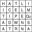
Players are then given a certain amount of time during which they
compete to try to form as many unique words as they can from these
letters. The letters of a word must be adjacent either horizontally,
vertically, or diagonally, and no die may be used more than once in a
single word. There is a minimum word length, and longer words are worth
more points. For example, the above game board contains the words,
“WITCH”, “ITCH”, “PELLET”, “TELL”, and “DATA”, among many others.
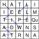
Suppose we want to build a program that plays Boggle against a human
opponent. The program would need to look for words on a given board. The
dictionary of valid words can of course be stored in a trie. In what follows,
we will show how the structure of a trie can be particularly helpful in
guiding this search so that words are found more quickly.
We can think of a search from a given starting point as a traversal of a
tree. The root of the tree is the starting point, and its children are
searches starting from adjacent dice. We must be careful, however, to
include in such a tree only those adjacent dice that do not already
occur on the path to the given die. For example, if we start a search at
the upper-left corner of the above board, its children would be the
three adjacent dice containing “I”, “C”, and “A”. The children of “I”,
then, would not include “H” because it is already on the path to “I”.
Part of this tree would look like this:
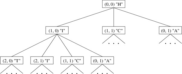
Note that this tree is not a data structure - it need not be explicitly
stored anywhere. Rather, it is a mathematical object that helps us to
design an algorithm for finding all of the words. Each word on the board
is simply a path in this tree starting from the root. We can therefore
traverse this tree in much the same way as we outlined in the previous
section
for tries.
For each node in the tree, we can look up the path leading to that node,
and output it if it is a word in the dictionary.
In order to be able to implement such a traversal, we need to be able to
find the children of a node. These children are the adjacent cells that
are not used in the path to the node. An efficient way to keep track of
the cells used in this path is with a bool[ , ] of the same
size as the Boggle board - a value of true in this array will
indicate that the corresponding cell on the board has been used in the
current path. The children of a node are then the adjacent cells whose
entries in this array are false.
A preorder traversal of this tree will therefore need the following
parameters (and possibly others, depending on how we want to output the
words found):
- The row index of the current cell.
- The column index of the current cell.
- The bool[ , ] described above. The current cell will
have a false entry in this array.
- A StringBuilder giving the letters on the path up to, but not
including, the current cell.
The preorder traversal will first need to update the cells used by
setting the location corresponding to the current cell to true.
Likewise, it will need to update the StringBuilder by appending the
contents of the current cell. Then it will need to process the root by
looking up the contents of the StringBuilder - if this forms a word,
it should output this word. Then it should process the children: for
each adjacent cell whose entry in the bool[ , ] is
false, it should make a recursive call on that cell. After all the
children have been processed, it will need to return the
bool[ , ] and the StringBuilder to their
earlier states by setting the array entry back to false and removing
the character(s) appended earlier.
Once such a method is written, we can call it once for each cell on the
board. For each of these calls, all entries in the bool[ , ]
should be false, and the StringBuilder should be empty.
While the algorithm described above will find all the words on a Boggle
board, a 5 x 5 board will require quite a while for the algorithm
to process. While this might be acceptable if we are implementing a game
that humans can compete with, from an algorithmic standpoint, we would
like to improve the performance. (In fact, there are probably better
ways to make a program with which humans can compete, as this search
will only find words that begin near the top of the board.)
We can begin to see how to improve the performance if we observe the
similarity between the trees we have been discussing and a trie
containing the word list. Consider, for example, a portion of the child
labeled ‘h’ in a trie representing a large set of words:
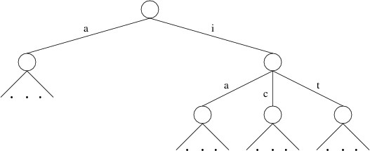
We have omitted some of the children because they are irrelevant to the
search we are performing (e.g., there is no die containing “E” adjacent
to “H” on the above game board). Also, we are assuming a minimum word
length of 4; hence, “ha”, “hi”, and “hit” are not shown as words in this
trie.
Notice the similarity between the trie portion shown above and the tree
shown earlier. The root of the tree has children representing dice
containing “I” and “A”, and the former node has children representing
dice containing “T”, “C”, and “A”; likewise, though they are listed in a
different order, the trie has children labeled ‘i’ and ‘a’, and the
former node has children labeled ’t’, ‘c’, and ‘a’.
What is more important to our discussion, however, is that the trie does
not have a child labeled ‘c’, as there is no English word beginning with
“hc”. Similarly, the child labeled ‘i’ does not have a child labeled
‘i’, as there is no English word beginning with “hii”. If there are no
words in the word list beginning with these prefixes, there is no need
to search the subtrees rooted at the corresponding nodes when doing the
preorder traversal. Using the trie to prune the search in this way ends
up avoiding many subtrees that don’t lead to any words. As a result,
only a small fraction of the original tree is searched.
In order to take advantage of the trie in this way, we need a method in
the trie implementation to return the child having a given label, or
null if there is no such child. Alternatively, we might provide a
method that takes a string and returns the trie that this string
leads to, or null if there is no such trie (this method would make
it easier to handle the die containing “Qu”). Either way, we can then
traverse the trie as we are doing the preorder traversal described
above, and avoid searching a subtree whenever the trie becomes null.
This revised preorder traversal needs an extra parameter - a trie giving
all completions of words beginning with the prefix given by the
StringBuilder parameter. We will need to ensure that this parameter
is never null. The algorithm then proceeds as follows:
- From the given trie, get the subtrie containing the completions of
words beginning with the contents of the current cell.
- If this subtrie is not null:
- Set the location in the bool[ , ] corresponding to
the current cell to true.
- Append the contents of the current cell to the
StringBuilder.
- If the subtrie obtained above contains the empty string,
output the contents of the StringBuilder as a word found.
- Recursively traverse each adjacent cell whose corresponding
entry in the bool[ , ] is false. The recursive
calls should use the subtrie obtained above.
- Set the location in the bool[ , ] corresponding to
the current cell to false.
- Remove the contents of the current cell from the end of the
StringBuilder (i.e., decrease its Length by the
appropriate amount).
We would then apply the above algorithm to each cell on the board. For
each cell, we would use a bool[ , ] whose entries are all
false, an empty StringBuilder, and the entire trie of valid words. Note that we
have designed the preorder traversal so that it leaves each of these
parameters unchanged; hence, we only need to initialize them once. The
resulting search will find all of the words on the board quickly.
Subsections of Priority Queues
Heaps
Heaps
A common structure for implementing a priority queue is known as a
heap. A heap is a tree whose nodes contain elements with priorities
that can be ordered. Furthermore, if the heap is nonempty, its root
contains the maximum priority of any node in the heap, and each of its
children is also a heap. Note that this implies that, in any subtree,
the maximum priority is at the root. We define a min-heap similarly,
except that the minimum priority is at the root. Below is an example of
a min-heap with integer priorities (the data elements are not shown —
only their priorities):
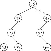
Note that this structure is different from a binary search tree, as
there are elements in the left child that have larger priorities than
the root. Although some ordering is imposed on the nodes (i.e.,
priorities do not decrease as we go down a path from the root), the
ordering is less rigid than for a binary search tree. As a result, there
is less overhead involved in maintaining this ordering; hence, a
min-heap tends to give better performance than an AVL tree, which could
also be used to implement a min-priority queue. Although the definition
of a heap does not require it, the implementations we will consider will
be binary trees, as opposed to trees with an arbitrary number of
children.
Note
The heap data structure is
unrelated to the pool of memory from which instances of reference types
are constructed — this also, unfortunately, is called a heap.
One advantage to using a min-heap to implement a min-priority queue is
fairly obvious — an element with minimum priority is always at the root
if the min-heap is nonempty. This makes it easy to find the minimum
priority and an element with this priority. Let’s consider how we might
remove an element with minimum priority. Assuming the min-heap is
nonempty, we need to remove the element at the root. Doing so leaves us
with two min-heaps (either of which might be empty). To complete the
removal, we need a way to merge two min-heaps into one. Note that if we
can do this, we also have a way of adding a new element: we form a
1-node min-heap from the new element and its priority, then merge this
min-heap with the original one.
Let us therefore consider the problem of merging two min-heaps into one.
If either min-heap is empty, we can simply use the other one. Suppose
that both are nonempty. Then the minimum priority of each is located at
its root. The minimum priority overall must therefore be the smaller of
these two priorities. Let s denote the heap whose root has the smaller
priority and b denote the heap whose root has the larger priority.
Then the root of s should be the root of the resulting min-heap.
Now that we have determined the root of the result, let’s consider what
we have left. s has two children, both of which are min-heaps, and b
is also a min-heap. We therefore have three min-heaps, but only two
places to put them - the new left and right children of s. To reduce
the number of min-heaps to two, we can merge two of them into one. This
is simply a recursive call.
We have therefore outlined a general strategy for merging two min-heaps.
There two important details that we have omitted, though:
- Which two min-heaps do we merge in the recursive call?
- Which of the two resulting min-heaps do we make the new left child
of the new root?
There are various ways these questions can be answered. Some ways lead
to efficient implementations, whereas others do not. For example, if we
always merge the right child of s with b and make the result the new
right child of the new root, it turns out that all of our min-heaps will have
empty left children. As a result, in the worst case, the time needed to
merge two min-heaps is proportional to the total number of elements in
the two min-heaps. This is poor performance. In the next
section
we will
consider a specific implementation that results in a worst-case running
time proportional to the logarithm of the total number of nodes.
Leftist Heaps
Leftist Heaps
One efficient way to complete the merge algorithm outlined in the
previous section
revolves
around the concept of the null path length of a tree. For any tree t, null path length of t is defined
to be
$ 0 $ if t is empty, or one more than the minimum of the null path
lengths of its children if t is nonempty. Another way to understand
this concept is that it gives the minimum number of steps needed to get
from the root to an empty subtree. For an empty tree, there is no root,
so we somewhat arbitrarily define the null path length to be
$ 0 $. For
single-node trees or binary trees with at least one empty child, the
null path length is
$ 1 $ because only one step is needed to reach an empty
subtree.
One reason that the null path length is important is that it can be
shown that any binary tree with
$ n $ nodes has a null path length that is
no more than
$ \lg(n + 1) $. Furthermore, recall that in the merging
strategy outlined in the previous
section
, there is some
flexibility in choosing which child of a node will be used in the
recursive call. Because the strategy reaches a base case when one of the
min-heaps is empty, the algorithm will terminate the most quickly if we
do the recursive call on the child leading us more quickly to an empty
subtree — i.e., if we use the child with smaller null path length.
Because this length is logarithmic in the number of nodes in the
min-heap, this choice will quickly lead us to the base case and
termination.
A common way of implementing this idea is to use what is known as a
leftist heap. A leftist heap is a binary tree that forms a heap such
that for every node, the null path length of the right child is no more
than the null path length of the left child. For such a structure,
completing the merge algorithm is simple:
- For the recursive call, we merge the right child of s with b,
where s and b are as defined in the previous
section
.
- When combining the root and left child of s with the result of the
recursive call, we arrange the children so that the result is a
leftist heap.
We can implement this idea by defining two classes, LeftistTree<T>
and MinPriorityQueue<TPriority, TValue>. For the
LeftistTree<T> class, we will only be concerned with the shape of
the tree — namely, that the null path length of the right child is never
more than the null path length of the left child. We will adopt a
strategy similar to what we did with AVL
trees
. Specifically a
LeftistTree<T> will be immutable so that we can always be sure
that it is shaped properly. It will then be a straightforward matter to
implement a MinPriorityQueue<TPriority, TValue>, where
TPriority is the type of the priorities, and TValue is the type
of the values.
The implementation of LeftistTree<T> ends up being very similar to
the implementation we described for AVL tree
nodes
, but without the
rotations. We need three public properties using the default
implementation with get accessors: the data (of type T) and the
two children (of type LeftistTree<T>?). We also need a private
field to store the null path length (of type int). We can define a
static method to obtain the null path length of a given
LeftistTree<T>?. This method is essentially the same as the
Height method for an AVL tree, except that if the given tree is
null, we return 0. A constructor takes as its parameters a data
element of type T and two children of type LeftistTree<T>?. It
can initialize its data with the first parameter. To initialize its
children, it first needs to determine their null path lengths using the
static method above. It then assigns the two LeftistTree<T>?
parameters to its child fields so that the right child’s null path
length is no more than the left child’s. Finally, it can initialize its
own null path length by adding 1 to its right child’s null path length.
Let’s now consider how we can implement
MinPriorityQueue<TPriority, TValue>. The first thing we need to
consider is the type, TPriority. This needs to be a non-nullable type that can be
ordered (usually it will be a numeric type like int). We can
restrict TPriority to be a non-nullable subtype of IComparable<TPriority>
by using a where clause, as we did for dictionaries (see
“Implementing a Dictionary with a Linked
List
”).
We then need a private field in which to store a leftist tree. We
can store both the priority and the data element in a node if we use a
LeftistTree<KeyValuePair<TPriority, TValue>>?; thus, the keys are
the priorities and the values are the data elements. We also need a
public int property to get of the number of elements in the
min-priority queue. This property can use the default implementation
with get and private set accessors.
In order to implement public methods to add an element with a
priority and to remove an element with minimum priority, we need the
following method:
private static LeftistTree<KeyValuePair<TPriority, TValue>>?
    Merge(LeftistTree<KeyValuePair<TPriority, TValue>>? h1,
        LeftistTree<KeyValuePair<TPriority, TValue>>? h2)
{
    . . .
}
This method consist of three cases. The first two cases occur when
either of the parameters is null. In each such case, we return the
other parameter. In the third case, when neither parameter is null,
we first need to compare the priorities in the data stored in the root
nodes of the parameters. A priority is stored in the
Key
property of the KeyValuePair, and we have constrained this type so
that it has a CompareTo method that will compare one instance with
another. Once we have determined which root has a smaller priority, we
can construct and return a new
LeftistTree<KeyValuePair<TPriority, TValue>> whose data
is the data element with smaller priority, and whose children are the
left child of this data element and the result of recursively merging
the right child of this element with the parameter whose root has larger
priority.
The remaining methods and properties of
MinPriorityQueue<TPriority, TValue> are now fairly
straightforward.
Huffman Trees
Huffman Trees
In this section, we’ll consider an application of min-priority queues to
the general problem of compressing files. Consider, for example, a plain
text file like this copy of the U. S. Constitution
. This file
is encoded using UTF-8, the most common encoding for plain text files.
The characters most commonly appearing in English-language text files
are each encoded as one byte (i.e., eight bits) using this scheme. For
example, in the text file referenced above, every character is encoded
as a single byte (the first three bytes of the file are an optional code
indicating that it is encoded in UTF-8 format). Furthermore, some byte
values occur much more frequently than others. For example, the encoding
of the blank character occurs over 6000 times, whereas the encoding of
‘$’ occurs only once, and the encoding of ‘=’ doesn’t occur at all.
One of the techniques used by most file compression schemes is to find a
variable-width encoding scheme for the file. Such a scheme uses fewer
bits to encode commonly-occurring byte values and more bits to encode
rarely-occurring byte values. Byte values that do not occur at all in
the file are not given an encoding.
Consider, for example, a file containing the single string,
“Mississippi”, with no control characters signaling the end of the line.
If we were to use one byte for each character, as UTF-8 would do, we
would need 11 bytes (or 88 bits). However, we could encode the
characters in binary as follows:
Obviously because each character is encoded with fewer than 8 bits, this
will give us a shorter encoding. However, because ‘i’ and ’s’, which
each occur four times in the string, are given shorter encodings than
‘M’ and ‘p’, which occur a total of three times combined, the number of
bits is further reduced. The encoded string is
100011110111101011010
which is only 21 bits, or less than 3 bytes.
In constructing such an encoding scheme, it is important that the
encoded string can be decoded unambiguously. For example, it would
appear that the following scheme might be even better:
This scheme produces the following encoding:
01011011010100
which is only 14 bits, or less than 2 bytes. However, when we try to
decode it, we immediately run into problems. Is the first 0 an ‘i’ or
the first bit of an ‘M’? We could decode this string as “isMsMsMisii”,
or a number of other possible strings.
The first encoding above, however, has only one decoding, “Mississippi”.
The reason for this is that this encoding is based on the following
binary tree:
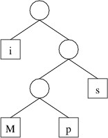
To get the encoding for a character, we trace the path to that character
from the root, and record a 0 each time we go left and a 1 each time we
go right. Thus, because the path to ‘M’ is right, left, left, we have an
encoding of 100. To decode, we simply use the encoding to trace out a
path in the tree, and when we reach a character (or more generally, a
byte value), we record that value. If we form the tree such that each
node has either two empty children or two nonempty children, then when
tracing out a path, we will always either have a choice of two
alternatives or be at a leaf storing a byte value. The decoding will
therefore be unambiguous. Such a tree that gives an encoding whose
length is minimized over all such encodings is called a Huffman tree.
Before we can find a Huffman tree for a file, we need to determine how
many times each byte value occurs. There are 256 different byte values
possible; hence we will need an array of 256 elements to keep track of
the number of occurrences of each. Because files can be large, this
array should be a long[ ]. We can then use element i of this
array to keep track of the number of occurrences of byte value i.
Thus, after constructing this array, we can read the file one byte at a
time as described in “Other File
I/O”
, and for each
byte b that we read, we increment the value at location b of the
array.
Having built this frequency table, we can now use it to build a Huffman
tree. We will build this tree from the bottom up, storing subtrees in a
min-priority queue. The priority of each subtree will be the total
number of occurrences of all the byte values stored in its leaves. We
begin by building a 1-node tree from each nonzero value in the frequency
table. As we iterate through the frequency table, if we find that
location i is nonzero, we construct a node containing i and add that
node to the min-priority queue. The priority we use when adding the node
is the number of occurrences of i, which is simply the value at
location i of the frequency table.
Once the min-priority queue has been loaded with the leaves, can begin
combining subtrees into larger trees. We will need to handle as a
special case an empty min-priority queue, which can result only from an
empty input file. In this case, there is no Huffman tree, as there are
no byte values that need to be encoded. Otherwise, as long as the
min-priority queue has more than one element, we:
- Get and remove the two smallest priorities and their associated
trees.
- Construct a new binary tree with these trees as its children and 0
as its data (which will be unused).
- Add the resulting tree to the min-priority queue with a priority
equal to the sum of the priorities of its children.
Because each iteration removes two elements from the min-priority queue
and adds one, eventually the min-priority queue will contain only one
element. It can be shown that this last remaining element is a Huffman
tree for the file.
Most file compression schemes involve more than just converting to a
Huffman-tree encoding. Furthermore, even if this is the only technique
used, simply writing the encoded data is insufficient to compress the
file, as the Huffman tree is needed to decompress it. Therefore, some
representation of the Huffman tree must also be written. In addition, a
few extra bits may be needed to reach a byte boundary. Because of this,
the length of the decompressed file is also needed for decompression so
that the extra bits are not interpreted as part of the encoded data. Due
to this additional output, compressing a short file will likely result
in a longer file than the original.