Heaps

A common structure for implementing a priority queue is known as a heap. A heap is a tree whose nodes contain elements with priorities that can be ordered. Furthermore, if the heap is nonempty, its root contains the maximum priority of any node in the heap, and each of its children is also a heap. Note that this implies that, in any subtree, the maximum priority is at the root. We define a min-heap similarly, except that the minimum priority is at the root. Below is an example of a min-heap with integer priorities (the data elements are not shown — only their priorities):

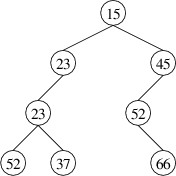
Note that this structure is different from a binary search tree, as there are elements in the left child that have larger priorities than the root. Although some ordering is imposed on the nodes (i.e., priorities do not decrease as we go down a path from the root), the ordering is less rigid than for a binary search tree. As a result, there is less overhead involved in maintaining this ordering; hence, a min-heap tends to give better performance than an AVL tree, which could also be used to implement a min-priority queue. Although the definition of a heap does not require it, the implementations we will consider will be binary trees, as opposed to trees with an arbitrary number of children.

One advantage to using a min-heap to implement a min-priority queue is fairly obvious — an element with minimum priority is always at the root if the min-heap is nonempty. This makes it easy to find the minimum priority and an element with this priority. Let’s consider how we might remove an element with minimum priority. Assuming the min-heap is nonempty, we need to remove the element at the root. Doing so leaves us with two min-heaps (either of which might be empty). To complete the removal, we need a way to merge two min-heaps into one. Note that if we can do this, we also have a way of adding a new element: we form a 1-node min-heap from the new element and its priority, then merge this min-heap with the original one.

Let us therefore consider the problem of merging two min-heaps into one. If either min-heap is empty, we can simply use the other one. Suppose that both are nonempty. Then the minimum priority of each is located at its root. The minimum priority overall must therefore be the smaller of these two priorities. Let s denote the heap whose root has the smaller priority and b denote the heap whose root has the larger priority. Then the root of s should be the root of the resulting min-heap.

Now that we have determined the root of the result, let’s consider what we have left. s has two children, both of which are min-heaps, and b is also a min-heap. We therefore have three min-heaps, but only two places to put them - the new left and right children of s. To reduce the number of min-heaps to two, we can merge two of them into one. This is simply a recursive call.

We have therefore outlined a general strategy for merging two min-heaps. There two important details that we have omitted, though:

• Which two min-heaps do we merge in the recursive call?
• Which of the two resulting min-heaps do we make the new left child of the new root?

There are various ways these questions can be answered. Some ways lead to efficient implementations, whereas others do not. For example, if we always merge the right child of s with b and make the result the new right child of the new root, it turns out that all of our min-heaps will have empty left children. As a result, in the worst case, the time needed to merge two min-heaps is proportional to the total number of elements in the two min-heaps. This is poor performance. In the next section we will consider a specific implementation that results in a worst-case running time proportional to the logarithm of the total number of nodes.

Leftist Heaps

One efficient way to complete the merge algorithm outlined in the previous section revolves around the concept of the null path length of a tree. For any tree t, null path length of t is defined to be $ 0 $ if t is empty, or one more than the minimum of the null path lengths of its children if t is nonempty. Another way to understand this concept is that it gives the minimum number of steps needed to get from the root to an empty subtree. For an empty tree, there is no root, so we somewhat arbitrarily define the null path length to be $ 0 $. For single-node trees or binary trees with at least one empty child, the null path length is $ 1 $ because only one step is needed to reach an empty subtree.

One reason that the null path length is important is that it can be shown that any binary tree with $ n $ nodes has a null path length that is no more than $ \lg(n + 1) $. Furthermore, recall that in the merging strategy outlined in the previous section , there is some flexibility in choosing which child of a node will be used in the recursive call. Because the strategy reaches a base case when one of the min-heaps is empty, the algorithm will terminate the most quickly if we do the recursive call on the child leading us more quickly to an empty subtree — i.e., if we use the child with smaller null path length. Because this length is logarithmic in the number of nodes in the min-heap, this choice will quickly lead us to the base case and termination.

A common way of implementing this idea is to use what is known as a leftist heap. A leftist heap is a binary tree that forms a heap such that for every node, the null path length of the right child is no more than the null path length of the left child. For such a structure, completing the merge algorithm is simple:

• For the recursive call, we merge the right child of s with b, where s and b are as defined in the previous section .
• When combining the root and left child of s with the result of the recursive call, we arrange the children so that the result is a leftist heap.

We can implement this idea by defining two classes, LeftistTree<T> and MinPriorityQueue<TPriority, TValue>. For the LeftistTree<T> class, we will only be concerned with the shape of the tree — namely, that the null path length of the right child is never more than the null path length of the left child. We will adopt a strategy similar to what we did with AVL trees . Specifically a LeftistTree<T> will be immutable so that we can always be sure that it is shaped properly. It will then be a straightforward matter to implement a MinPriorityQueue<TPriority, TValue>, where TPriority is the type of the priorities, and TValue is the type of the values.

The implementation of LeftistTree<T> ends up being very similar to the implementation we described for AVL tree nodes , but without the rotations. We need three public properties using the default implementation with get accessors: the data (of type T) and the two children (of type LeftistTree<T>?). We also need a private field to store the null path length (of type int). We can define a static method to obtain the null path length of a given LeftistTree<T>?. This method is essentially the same as the Height method for an AVL tree, except that if the given tree is null, we return 0. A constructor takes as its parameters a data element of type T and two children of type LeftistTree<T>?. It can initialize its data with the first parameter. To initialize its children, it first needs to determine their null path lengths using the static method above. It then assigns the two LeftistTree<T>? parameters to its child fields so that the right child’s null path length is no more than the left child’s. Finally, it can initialize its own null path length by adding 1 to its right child’s null path length.

Let’s now consider how we can implement MinPriorityQueue<TPriority, TValue>. The first thing we need to consider is the type, TPriority. This needs to be a non-nullable type that can be ordered (usually it will be a numeric type like int). We can restrict TPriority to be a non-nullable subtype of IComparable<TPriority> by using a where clause, as we did for dictionaries (see “Implementing a Dictionary with a Linked List ”).

We then need a private field in which to store a leftist tree. We can store both the priority and the data element in a node if we use a LeftistTree<KeyValuePair<TPriority, TValue>>?; thus, the keys are the priorities and the values are the data elements. We also need a public int property to get of the number of elements in the min-priority queue. This property can use the default implementation with get and private set accessors.

In order to implement public methods to add an element with a priority and to remove an element with minimum priority, we need the following method:

private static LeftistTree<KeyValuePair<TPriority, TValue>>?
    Merge(LeftistTree<KeyValuePair<TPriority, TValue>>? h1, 
        LeftistTree<KeyValuePair<TPriority, TValue>>? h2)
{
    . . .
}

This method consist of three cases. The first two cases occur when either of the parameters is null. In each such case, we return the other parameter. In the third case, when neither parameter is null, we first need to compare the priorities in the data stored in the root nodes of the parameters. A priority is stored in the Key property of the KeyValuePair, and we have constrained this type so that it has a CompareTo method that will compare one instance with another. Once we have determined which root has a smaller priority, we can construct and return a new LeftistTree<KeyValuePair<TPriority, TValue>> whose data is the data element with smaller priority, and whose children are the left child of this data element and the result of recursively merging the right child of this element with the parameter whose root has larger priority.

The remaining methods and properties of MinPriorityQueue<TPriority, TValue> are now fairly straightforward.

Huffman Trees

In this section, we’ll consider an application of min-priority queues to the general problem of compressing files. Consider, for example, a plain text file like this copy of the U. S. Constitution . This file is encoded using UTF-8, the most common encoding for plain text files. The characters most commonly appearing in English-language text files are each encoded as one byte (i.e., eight bits) using this scheme. For example, in the text file referenced above, every character is encoded as a single byte (the first three bytes of the file are an optional code indicating that it is encoded in UTF-8 format). Furthermore, some byte values occur much more frequently than others. For example, the encoding of the blank character occurs over 6000 times, whereas the encoding of ‘$’ occurs only once, and the encoding of ‘=’ doesn’t occur at all.

One of the techniques used by most file compression schemes is to find a variable-width encoding scheme for the file. Such a scheme uses fewer bits to encode commonly-occurring byte values and more bits to encode rarely-occurring byte values. Byte values that do not occur at all in the file are not given an encoding.

Consider, for example, a file containing the single string, “Mississippi”, with no control characters signaling the end of the line. If we were to use one byte for each character, as UTF-8 would do, we would need 11 bytes (or 88 bits). However, we could encode the characters in binary as follows:

• M: 100
• i: 0
• p: 101
• s: 11

Obviously because each character is encoded with fewer than 8 bits, this will give us a shorter encoding. However, because ‘i’ and ’s’, which each occur four times in the string, are given shorter encodings than ‘M’ and ‘p’, which occur a total of three times combined, the number of bits is further reduced. The encoded string is

100011110111101011010

which is only 21 bits, or less than 3 bytes.

In constructing such an encoding scheme, it is important that the encoded string can be decoded unambiguously. For example, it would appear that the following scheme might be even better:

• M: 01
• i: 0
• p: 10
• s: 1

This scheme produces the following encoding:

01011011010100

which is only 14 bits, or less than 2 bytes. However, when we try to decode it, we immediately run into problems. Is the first 0 an ‘i’ or the first bit of an ‘M’? We could decode this string as “isMsMsMisii”, or a number of other possible strings.

The first encoding above, however, has only one decoding, “Mississippi”. The reason for this is that this encoding is based on the following binary tree:

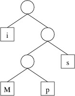
To get the encoding for a character, we trace the path to that character from the root, and record a 0 each time we go left and a 1 each time we go right. Thus, because the path to ‘M’ is right, left, left, we have an encoding of 100. To decode, we simply use the encoding to trace out a path in the tree, and when we reach a character (or more generally, a byte value), we record that value. If we form the tree such that each node has either two empty children or two nonempty children, then when tracing out a path, we will always either have a choice of two alternatives or be at a leaf storing a byte value. The decoding will therefore be unambiguous. Such a tree that gives an encoding whose length is minimized over all such encodings is called a Huffman tree.

Before we can find a Huffman tree for a file, we need to determine how many times each byte value occurs. There are 256 different byte values possible; hence we will need an array of 256 elements to keep track of the number of occurrences of each. Because files can be large, this array should be a long[ ]. We can then use element i of this array to keep track of the number of occurrences of byte value i. Thus, after constructing this array, we can read the file one byte at a time as described in “Other File I/O” , and for each byte b that we read, we increment the value at location b of the array.

Having built this frequency table, we can now use it to build a Huffman tree. We will build this tree from the bottom up, storing subtrees in a min-priority queue. The priority of each subtree will be the total number of occurrences of all the byte values stored in its leaves. We begin by building a 1-node tree from each nonzero value in the frequency table. As we iterate through the frequency table, if we find that location i is nonzero, we construct a node containing i and add that node to the min-priority queue. The priority we use when adding the node is the number of occurrences of i, which is simply the value at location i of the frequency table.

Once the min-priority queue has been loaded with the leaves, can begin combining subtrees into larger trees. We will need to handle as a special case an empty min-priority queue, which can result only from an empty input file. In this case, there is no Huffman tree, as there are no byte values that need to be encoded. Otherwise, as long as the min-priority queue has more than one element, we:

• Get and remove the two smallest priorities and their associated trees.
• Construct a new binary tree with these trees as its children and 0 as its data (which will be unused).
• Add the resulting tree to the min-priority queue with a priority equal to the sum of the priorities of its children.

Because each iteration removes two elements from the min-priority queue and adds one, eventually the min-priority queue will contain only one element. It can be shown that this last remaining element is a Huffman tree for the file.

Most file compression schemes involve more than just converting to a Huffman-tree encoding. Furthermore, even if this is the only technique used, simply writing the encoded data is insufficient to compress the file, as the Huffman tree is needed to decompress it. Therefore, some representation of the Huffman tree must also be written. In addition, a few extra bits may be needed to reach a byte boundary. Because of this, the length of the decompressed file is also needed for decompression so that the extra bits are not interpreted as part of the encoded data. Due to this additional output, compressing a short file will likely result in a longer file than the original.