Select Sorts

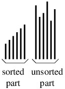
A select sort operates by repeatedly selecting the smallest data element of an unsorted portion of the array and moving it to the end of a sorted portion. Thus, at each step, the data items will be arranged into two parts:

1. A sorted part; and
2. An unsorted part in which each element is at least as large as all elements in the sorted part.

The following figure illustrates this arrangement.

Initially, the sorted part will be empty. At each step, the unsorted part is rearranged so that its smallest element comes first. As a result, the sorted part can now contain one more element, and the unsorted part one fewer element. After $ n - 1 $ steps, where $ n $ is the number of elements in the array, the sorted part will have all but one of the elements. Because the one element in the unsorted part must be at least as large as all elements in the sorted part, the entire array will be sorted at this point.

The approach outlined above can be implemented in various ways. The main difference in these implementations is in how we rearrange the unsorted part to bring its smallest element to the beginning of that part. The most straightforward way to do this is to find the smallest element in this part, then swap it with the first element in this part. The resulting algorithm is called selection sort. It requires nested loops. The outer loop index keeps track of how many elements are in the sorted part. The unsorted part then begins at this index. The inner loop is responsible for finding the smallest element in the unsorted part. Once the inner loop has finished, the smallest element is swapped with the first element in the unsorted part.

Note that the inner loop in selection sort iterates once for every element in the unsorted part. On the first iteration of the outer loop, the unsorted part contains all $ n $ elements. On each successive iteration, the unsorted part is one element smaller, until on the last iteration, it has only $ 2 $ elements. If we add up all these values, we find that the inner loop iterates a total of exactly $ (n - 1)(n + 2)/2 $ times. This value is proportional to $ n^2 $ as $ n $ increases; hence, the running time of the algorithm is in $ O(n^2) $. Furthermore, this performance occurs no matter how the data items are initially arranged.

As we will see in what follows, $ O(n^2) $ performance is not very good if we want to sort a moderately large data set. For example, sorting $ 100,000 $ elements will require about $ 5 $ billion iterations of the inner loop. On the positive side, the only time data items are moved is when a swap is made at the end of the outer loop; hence, this number is proportional to $ n $. This could be advantageous if we are sorting large value types, as we would not need to write these large data elements very many times. However, for general performance reasons, large data types shouldn’t be value types — they should be reference types to avoid unnecessary copying of the values. For this reason, selection sort isn’t a particularly good sorting algorithm.

Performance issues aside, however, there is one positive aspect to selection sort. This aspect has to do with sorting by keys. Consider, for example, the rows of a spreadsheet. We often want to sort these rows by the values in a specific column. These values are the sort keys of the elements. In such a scenario, it is possible that two data elements are different, but their sort keys are the same. A sorting algorithm might reverse the order of these elements, or it might leave their order the unchanged. In some cases, it is advantageous for a sorting algorithm to leave the order of these elements unchanged. For example, if we sort first by a secondary key, then by a primary key, we would like for elements whose primary keys are equal to remain sorted by their secondary key. Therefore, a sorting algorithm that always maintains the original order of equal keys is said to be stable. If we are careful how we implement the inner loop of selection sort so that we always select the first instance of the smallest key, then this algorithm is stable.

Another implementation of a select sort is bubble sort. It rearranges the unsorted part by swapping adjacent elements that are out of order. It starts with the last two elements (i.e., the elements at locations $ n - 1 $ and $ n - 2 $), then the elements at locations $ n - 2 $ and $ n - 3 $, etc. Proceeding in this way, the smallest element in the unsorted part will end up at the beginning of the unsorted part. While the inner loop is doing this, it keeps track of whether it has made any swaps. If the loop completes without having made any swaps, then the array is sorted, and the algorithm therefore stops.

Like selection sort, bubble sort is stable. In the worst case, however, the performance of bubble sort is even worse than that of selection sort. It is still in $ O(n^2) $, but in the worst case, its inner loop performs the same number of iterations, but does a lot more swaps. Bubble sort does outperform selection sort on some inputs, but describing when this will occur isn’t easy. For example, in an array in which the largest element occurs in the first location, and the remaining locations are sorted, the performance ends up being about the same as selection sort — even though this array is nearly sorted. Like selection sort, it is best to avoid bubble sort.

A select sort that significantly outperforms selection sort is known as heap sort. This algorithm is based on the idea that a priority queue can be used to sort data — we first place all items in a priority queue, using the values themselves as priorities (if we are sorting by keys, then we use the keys as priorities). We then repeatedly remove the element with largest priority, filling the array from back to front with these elements.

We can optimize the above algorithm by using a priority queue implementation called a binary heap, whose implementation details we will only sketch. The basic idea is that we can form a binary tree from the elements of an array by using their locations in the array. The first element is the root, its children are the next two elements, their children are the next four elements, etc. Given an array location, we can then compute the locations of its parent and both of its children. The priorities are arranged so that the root of each subtree contains the maximum priority in that subtree. It is possible to arrange the elements of an array into a binary heap in $ O(n) $ time, and to remove an element with maximum priority in $ O(\lg n) $ time.

Heap sort then works by pre-processing the array to arrange it into a binary heap. The binary heap then forms the unsorted part, and it is followed by the sorted part, whose elements are all no smaller than any element in the unsorted part. While this arrangement is slightly different from the arrangement for the first two select sorts, the idea is the same. To rearrange the unsorted part, it:

1. Copies the first (i.e., highest-priority) element to a temporary variable.
2. Removes the element with maximum priority (i.e., the first element).
3. Places the copy of the first element into the space vacated by its removal at the beginning of the sorted part.

Heap sort runs in $ O(n \lg n) $ time in the worst case. Information theory can be used to prove that any sorting algorithm that sorts by comparing elements must make at least $ \lg(n!) $ comparisons on some arrays of size $ n $. Because $ \lg(n!) $ is proportional to $ n \lg n $, we cannot hope to do any better than $ O(n \lg n) $ in the worst case. While this performance is a significant improvement over selection sort and bubble sort, we will see in later that there is are algorithms that do even better in practice. Furthermore, heap sort is not stable.

On the other hand, we will also see that heap sort is an important component of an efficient hybrid algorithm. This algorithm is one of the best general-purpose sorting algorithms; in fact, it is used by .NET’s Array.Sort method. We will examine this approach in “Hybrid Sorts ”.

Insert Sorts

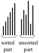
An insert sort operates by repeatedly inserting an element into a sorted portion of the array. Thus, as for select sorts, at each step the data items will be arranged into a sorted part, followed by an unsorted part; however, for insert sorts, there is no restriction on how elements in the unsorted part compare to elements in the sorted part. The following figure illustrates this arrangement.

Initially, the sorted part will contain the first element, as a single element is always sorted. At each step, the first element in the unsorted part is inserted into its proper location in the sorted part. As a result, the sorted part now contains one more element, and the unsorted part one fewer element. After $ n - 1 $ steps, where $ n $ is the number of elements in the array, the sorted part will contain all the elements, and the algorithm will be done.

Again, this approach can be implemented in various ways. The main difference in these implementations is in how we insert an element. The most straightforward way is as follows:

1. Copy the first element of the unsorted part to a temporary variable.
2. Iterate from the location of the first element of the unsorted part toward the front of the array as long as we are at an index greater than 0 and the element to the left of the current index is greater than the element in the temporary variable. On each iteration:
   • Copy the element to the left of the current index to the current index.
3. Place the value in the temporary variable into the location at which the above loop stopped.

The algorithm that uses the above insertion technique is known as insertion sort. Like selection sort, it requires an outer loop to keep track of the number of elements in the sorted part. Each iteration of this outer loop performs the above insertion algorithm. It is not hard to see that this algorithm is stable .

The main advantage insertion sort has over selection sort is that the inner loop only iterates as long as necessary to find the insertion point. In the worst case, it will iterate over the entire sorted part. In this case, the number of iterations is the same as for selection sort; hence, the worst-case running time is in $ O(n^2) $ — the same as selection sort and bubble sort . At the other extreme, however, if the array is already sorted, the inner loop won’t need to iterate at all. In this case, the running time is in $ O(n) $, which is the same as the running time of bubble sort on an array that is already sorted.

Unlike bubble sort, however, insertion sort has a clean characterization of its performance based on how sorted the array is. This characterization is based on the notion of an inversion, which is a pair of array locations $ i \lt j $ such that the value at location $ i $ is greater than the value at location $ j $; i.e., these two values are out of order with respect to each other. A sorted array has no inversions, whereas in an array of distinct elements in reverse order, every pair of locations is an inversion, for a total of $ n(n - 1)/2 $ inversions. In general, we can say that the fewer inversions an array has, the more sorted it is.

The reason why inversions are important to understanding the performance of insertion sort is that each iteration of the inner loop (i.e., step 2 of the insertion algorithm above) removes exactly one inversion. Consequently, if an array initially has $ k $ inversions, the inner loop will iterate a total of $ k $ times. If we combine this with the $ n - 1 $ iterations of the outer loop, we can conclude that the running time of insertion sort is in $ O(n + k) $. Thus, if the number of inversions is relatively small in comparison to $ n $ (i.e., the array is nearly sorted), insertion sort runs in $ O(n) $ time. (By contrast, $ n - 2 $ inversions can be enough to cause the inner loop of bubble sort to iterate its worst-case number of times.) For this reason, insertion sort is the algorithm of choice when we expect the data to be nearly sorted — a scenario that occurs frequently in practice. This fact is exploited by an efficient hybrid algorithm that combines insertion sort with two other sorting algorithms - see “Hybrid Sorting Algorithms ” for more details.

Before we consider another insert sort, there is one other advantage to insertion sort that we need to consider. Because the algorithm is simple (like selection sort and bubble sort), it performs well on small arrays. More complex algorithms like heap sort , while providing much better worst-case performance for larger arrays, don’t tend to perform as well on small arrays. In many cases, the performance difference on small arrays isn’t enough to matter, as pretty much any algorithm will perform reasonably well on a small array. However, this performance difference can become significant if we need to sort many small arrays (in a later section, we will see an application in which this scenario occurs). Because insertion sort tends to out-perform both selection sort and bubble sort, it is usually the best choice when sorting small arrays.

Another way to implement an insert sort is to use a balanced binary search tree, such as an AVL tree , to store the sorted part. In order to do this, we need to modify the definition of a binary search tree to allow multiple instances of the same key. In order to achieve stability, if we are inserting a key that is equal to a key already in the tree, we would treat the new key as being greater than the pre-existing key - i.e., we would recursively insert it into the right child. Once all the data items are inserted, we would then copy them back into the array in sorted order using an inorder traversal . We call this algorithm tree sort.

This algorithm doesn’t exactly match the above description of an insert sort, but it is not hard to see that it follows the same general principles. While the sorted portion is not a part of the array, but instead is a separate data structure, it does hold an initial part of the array in sorted order, and successive elements from the unsorted portion are inserted into it.

Because insertions into an AVL tree containing $ k $ elements can be done in $ O(\lg k) $ time in the worst case, and because an inorder traversal can be done in $ O(k) $ time, it follows that tree sort runs in $O(n \lg n)$ time in the worst case, where $ n $ is the number of elements in the array. However, because maintaining an AVL tree requires more overhead than maintaining a binary heap, heap sort tends to give better performance in practice. For this reason, tree sort is rarely used.

Merge Sorts

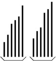
A merge sort works by merging together two sorted parts of an array. Thus, we should focus our attention on an array that is partitioned into two sorted parts, as shown in the following figure.

The different ways of implementing a merge sort depend both on how the above arrangement is achieved, and also on how the two parts are merged together. The simplest implementation is an algorithm simply called merge sort.

Merge sort uses recursion to arrange the array into two sorted parts. In order to use recursion, we need to express our algorithm, not in terms of sorting an array, but instead in terms of sorting a part of an array. If the part we are sorting has more than one element, then we can split it into two smaller parts of roughly equal size (if it doesn’t have more than one element, it is already sorted). Because both parts are smaller, we can recursively sort them to achieve the arrangement shown above.

The more complicated step in merge sort is merging the two sorted parts into one. While it is possible to do this without using another array (or other data structure), doing so is quite complicated. Merge sort takes a much simpler approach that uses a temporary array whose size is the sum of the sizes of the two sorted parts combined. It first accumulates the data items into the new array in sorted order, then copies them back into the original array.

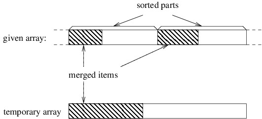
In order to understand how the merging works, let’s consider a snapshot of an arbitrary step of the algorithm. If we’ve accumulated an initial portion of the result, these elements will be the smallest ones. Because both of the parts we are merging are sorted, these smallest elements must come from initial portions of these two parts, as shown below.

Initially, the three shaded areas above are all empty. In order to proceed, we need local variables to keep track of the first index in each of the three unshaded areas. We then iterate as long as both of the unshaded areas are nonempty. On each iteration, we want to place the next element into the temporary array. This element needs to be the smallest of the unmerged elements. Because both parts of the given array are sorted, the smallest unmerged element will be the first element from one of the two unshaded parts of this array — whichever one is smaller (for stability, we use the first if they are equal). We copy that element to the beginning of the unshaded portion of the temporary array, then update the local variables to reflect that we have another merged item.

The above loop will terminate as soon as we have merged all the data items from one of the two sorted parts; however, the other sorted part will still contain unmerged items. To finish merging to the temporary array, we just need to copy the remaining items to the temporary array. We can do this by first copying all remaining items from the first sorted part, then copying all remaining items from the second sorted part (one of these two copies will copy nothing because there will be no remaining items in one of the two sorted parts). Once all items have been merged into the temporary array, we copy all items back to the original array to complete the merge.

We won’t do a running time analysis here, but merge sort runs in $ O(n \lg n) $ time in the worst case. Furthermore, unlike heap sort , it is stable. Because it tends to perform better in practice than tree sort , it is a better choice when we need a stable sorting algorithm. In fact, it is the basis (along with insertion sort ) of a stable hybrid sorting algorithm that performs very well in practice. This algorithm, called Tim sort, is rather complicated; hence, we won’t describe it here. If we don’t need a stable sorting algorithm, though, there are other alternatives, as we shall see in the next two sections.

Another scenario in which a merge sort is appropriate occurs when we have a huge data set that will not fit into an array. In order to sort such a data set, we need to keep most of the data in files while keeping a relatively small amount within internal data structures at any given time. Because merging processes data items sequentially, it works well with files. There are several variations on how we might do this, but the basic algorithm is called external merge sort.

External merge sort uses four temporary files in addition to an input file and an output file. Each of these files will alternate between being used for input and being used for output. Furthermore, at any given time, one of the two files being used for input will be designated as the first input file, and the other will designated as the second input file. Similarly, at any given time, one of the two files being used for output will be designated as the current output file, and the other will be designated as the alternate output file.

The algorithm begins with an initialization step that uses the given unsorted data file as its input, and two of the temporary files as its output. We will need two variables storing references to the current output file and the alternate output file, respectively. At this point we begin a loop that iterates until we reach the end of the input. Each iteration of this loop does the following:

1. Fill a large array with data items from the input (if there aren’t enough items to fill this array, we just use part of it).
2. Sort this array using whatever sorting algorithm is appropriate.
3. Write each element of the sorted array to the current output file.
4. Write a special end marker to the output file.
5. Swap the contents of the variables referring to the current output file and the alternate output file.

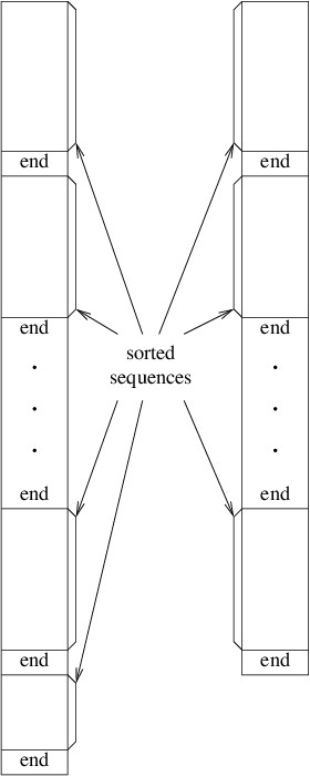
After the above loop terminates, the two output files are closed. Thus, the initialization writes several sorted sequences, each terminated by end markers, to the two output files. Furthermore, either the two output files will contain the same number of sorted sequences or the one that was written to first will contain one more sorted sequence than the other. The following figure illustrates these two files.

The algorithm then enters the main loop. Initially the output file first written in the initialization is designated as the first input file, and the other file written in the initialization is designated as the second input file. The other two temporary files are arbitrarily designated as the current output file and the alternate output file. The loop then iterates as long as the second input file is nonempty. Each iteration does the following:

1. While there is data remaining in the second input file:
   1. Merge the next sorted sequence in the first input file with the next sorted sequence in the second input file, writing the result to the current output file (see below for details).
   2. Write an end marker to the current output file.
   3. Swap the current output file and the alternate output file.
2. If there is data remaining in the first input file:
   1. Copy the remaining data from the first input file to the current output file
   2. Write an end marker to the current output file.
   3. Swap the current output file and the alternate output file.
3. Close all four temporary files.
4. Swap the first input file with the alternate output file.
5. Swap the second input file with the current output file.

Each iteration therefore combines pairs of sorted sequences from the two input files, thus reducing the number of sorted sequences by about half. Because it alternates between the two output files, as was done in the initialization, either the two output files will end up with the same number of sequences, or the last one written (which will be the alternate output file following step 2) will have one more than the other. The last two steps therefore ensure that to begin the next iteration, if the the number of sequences in the two input files is different, the first input file has the extra sequence.

The loop described above finishes when the second input file is empty. Because the first input file will have no more than one more sorted sequence than the second input file, at the conclusion of the loop, it will contain a single sorted sequence followed by an end marker. The algorithm therefore concludes by copying the data from this file, minus the end marker, to the output file.

Let’s now consider more carefully the merge done in step 1a above. This merge is done in essentially the same way that the merge is done in the original merge sort; however, we don’t need to read in the entire sorted sequences to do it. Instead, all we need is the next item from each sequence. At each step, we write the smaller of the two, then read the next item from the appropriate input file. Because we only need these two data items at any time, this merge can handle arbitrarily long sequences.

For an external sorting algorithm, the most important measure of performance is the number of file I/O operations it requires, as these operations are often much more expensive than any other (depending, of course, on the storage medium). Suppose the initial input file has $ n $ data items, and suppose the array we use in the initialization step can hold $ m $ data items. Then the number of sorted sequences written by the initialization is $ n/m $, with any fractional part rounded up. Each iteration of the main loop then reduces the number of sorted sequences by half, with any fractional part again rounded up. The total number of iterations of the main loop is therefore $ \lg (n/m) $, rounding upward again. Each iteration of this loop makes one pass through the entire data set. In addition, the initialization makes one pass, and the final copying makes one pass. The total number of passes through the data is therefore $ \lg (n/m) + 2 $. For example, if we are sorting $ 10 $ billion data items using an array of size $ 1 $ million, we need $ \lg 10,000 + 2 $ passes, rounded up; i.e., we need $ 16 $ passes through the data.

Various improvements can be made to reduce the number of passes through the data. For example, we can avoid the final file copy if we use another mechanism for denoting the end of a sorted sequence. One alternative is to keep track of the length of each sequence in each file in a List<long>. If the temporary files are within the same directory as the output file, we can finish the sort by simply renaming the first input file, rather than copying it.

A more substantial improvement involves using more temporary files. $ k $-way external merge sort uses $ k $ input and $ k $ output files. Each merge then merges $ k $ sorted sequences into $ 1 $. This reduces the number of iterations of the main loop to $ \log_k (n/m) $. Using the fact that $ \log_{k^2} n = (\log_k n)/2 $, we can conclude that squaring $ k $ will reduce the number of passes through the data by about half. Thus, $ 4 $-way external merge sort will make about half as many passes through the data as $ 2 $-way external merge sort. The gain diminishes quickly after that, however, as we must increase $ k $ to $ 16 $ to cut the number of passes in half again.

Split Sorts

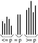
A split sort operates by splitting the array into three parts:

• An unsorted part containing elements less than or equal to some pivot element p.
• A nonempty part containing elements equal to p.
• An unsorted part containing elements greater than or equal to p.

This arrangement is illustrated in the following figure.

To complete the sort, it then sorts the two unsorted parts. Note that because the second part is nonempty, each of the two unsorted parts is smaller than the original data set; hence, the algorithm will always make progress.

The various implementations of a split sort are collectively known as quick sort. They differ in how many elements are placed in the middle part (only one element or all elements equal to the pivot), how the pivot is chosen, how the elements are partitioned into three parts, and how the two sub-problems are sorted. We will examine only two variations, which differ in how the pivot element is chosen.

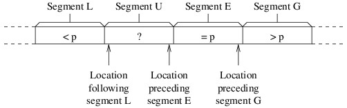
Let’s start with how we do the partitioning. Let p denote the pivot element. Because most of the split sort implementations use recursion to complete the sort, we’ll assume that we are sorting a portion of an array. At each stage of the partitioning, the array portion we are sorting will be arranged into the following four segments:

1. Segment L: Elements less than p.
2. Segment U: Elements we haven’t yet examined (i.e., unknown elements).
3. Segment E: Elements equal to p.
4. Segment G: Elements greater than p.

Initially, segments L, E, and G will be empty, and each iteration will reduce the size of segment U. The partitioning will be finished when segment U is empty. We will need three local variables to keep track of where one segment ends and another segment begins, as shown in the following figure:

We have worded the descriptions of the three local variables so that they make sense even if some of the segments are empty. Thus, because all segments except U are initially empty, the location following segment L will initially be the first location in the array portion that we are sorting, and the other two variables will initially be the last location in this portion. We then need a loop that iterates as long as segment U is nonempty — i.e., as long as the location following segment L is no greater than the location preceding segment E. Each iteration of this loop will compare the last element in segment U (i.e., the element at the location preceding segment E) with p. We will swap this element with another depending on how it compares with p:

• If it is less than p, we swap it with the element following segment L, and adjust the end of segment L to include it.
• If it is equal to p, we leave it where it is, and adjust the beginning of segment E to include it.
• If it is greater than p, we swap it with the element preceding segment G, adjust the beginning of segment G to include it, and adjust the beginning of segment E to account for the fact that we are shifting this segment to the left by 1.

Once this loop completes, the partitioning will be done. Furthermore, we can determine the two parts that need to be sorted from the final values of the local variables.

The first split sort implementation we will consider is fairly straightforward, given the above partitioning scheme. If we are sorting more than one element (otherwise, there is nothing to do), we will use as the pivot element the first element of the array portion to be sorted. After partitioning, we then sort the elements less than the pivot using a recursive call, and sort the elements greater than the pivot with another.

Though we won’t give an analysis here, the above algorithm runs in $ O(n^2) $ time in the worst case, where $ n $ is the number of elements being sorted. However, as we saw with insertion sort , the worst-case running time doesn’t always tell the whole story. Specifically, the expected running time of quick sort (this implementation and others) on random arrays is in $ O(n \lg n) $.

However, we don’t often need to sort random data. Let’s therefore take a closer look at what makes the worst case bad. In some ways this algorithm is like merge sort — it does two recursive calls, and the additional work is proportional to the number of elements being sorted. The difference is that the recursive calls in merge sort are both on array portions that are about half the size of the portion being sorted. With this quick sort implementation, on the other hand, the sizes of the recursive calls depend on how the first element (i.e., the pivot element) compares to the other elements. The more elements that end up in one recursive call, the slower the algorithm becomes. Consequently, the worst case occurs when the array is already sorted, and is still bad if the array is nearly sorted. For this reason, this is a particularly bad implementation.

Before we look at how we can improve the performance, we need to consider one other aspect of this implementation’s performance. For a recursive method, the amount of data pushed on the runtime stack is proportional to the depth of the recursion. In the worst cases (i.e., on a sorted array), the recursion depth is $ n $. Thus, for large $ n $, if the array is sorted or nearly sorted, a StackOverflowException is likely.

The most important thing we can do to improve the performance, in terms of both running time and stack usage, is to be more careful about how we choose the pivot element. We want to choose an element that partitions the data elements roughly in half. The median element (i.e., the element that belongs in the middle after the array is sorted) will therefore give us the optimal split. It is possible to design an $ O(n \lg n) $ algorithm that uses the median as the pivot; however, the time it takes to find the median makes this algorithm slower than merge sort in practice. It works much better to find a quick approximation for the median.

The main technique for obtaining such an approximation is to examine only a few of the elements. For example, we can use median-of-three partitioning, which uses as its pivot element the median of the first, middle, and last elements of the array portion we are sorting. An easy way to implement this strategy is to place these three elements in an array of size 3, then sort this array using insertion sort . The element that ends up at location 1 is then the used as the pivot.

We can improve on the above strategy by doing a case analysis of the three values. If we do this, we don’t need a separate array — we just find the median of three values, $ a $, $ b $, and $ c $, as follows:

• If $ a \lt b $:
  • If $ b \lt c $, then $ b $ is the median.
  • Otherwise, because $ b $ is the largest:
    • If $ a \lt c $, then $ c $ is the median.
    • Otherwise, $ a $ is the median.
• Otherwise, because $ b \leq a $:
  • If $ a \lt c $, then $ a $ is the median.
  • Otherwise, because $ a $ is the largest:
    • If $ b \lt c $, then $ c $ is the median.
    • Otherwise, $ b $ is the median.

The above algorithm is quite efficient, using at most three comparisons and requiring no values to be copied other than the result if we implement it in-line, rather than as a separate method (normally an optimizing compiler can do this method inlining for us). It also improves the sorting algorithm by tending to make the bad cases less likely.

This version of quick sort gives good performance most of the time, typically outperforming either heap sort or merge sort . However, it still has a worst-case running time in $ O(n^2) $ and a worst-case stack usage in $ O(n) $. Furthermore, it is unstable and does not perform as well as insertion sort on small or nearly sorted data sets. In the next section , we will show how quick sort can be combined with some of the other sorting algorithms to address some of these issues, including the bad worst-case performance.

Hybrid Sorting Algorithms

The best versions of quick sort are competitive with both heap sort and merge sort on the vast majority of inputs. However, quick sort has a very bad worst case — $ O(n^2) $ running time and $ O(n) $ stack usage. By comparison, both heap sort and merge sort have $ O(n \lg n) $ worst-case running time, together with a stack usage of $ O(1) $ for heap sort or $ O(\lg n) $ for merge sort. Furthermore, insertion sort performs better than any of these algorithms on small data sets. In this section, we look at ways to combine some of these algorithms to obtain a sorting algorithm that has the advantages of each of them.

We will start with quick sort, which gives the best performance for most inputs. One way of improving its performance is to make use of the fact that insertion sort is more efficient for small data sets. Improving the performance on small portions can lead to significant performance improvements for large arrays because quick sort breaks large arrays into many small portions. Hence, when the portion we are sorting becomes small enough, rather than finding a pivot and splitting, we instead call insertion sort.

An alternative to the above improvement is to use the fact that insertion sort runs in $ O(n) $ time when the number of inversions is linear in the number of array elements. To accomplish this, we modify quick sort slightly so that instead of sorting the array, it brings each element near where it belongs. We will refer to this modified algorithm as a partial sort. After we have done the partial sort, we then sort the array using insertion sort. The modification we make to quick sort to obtain the partial sort is simply to change when we stop sorting. We only sort portions that are larger than some threshold — we leave other portions unsorted.

Suppose, for example, that we choose a threshold of $ 10 $. Once the partial sort reaches an array portion with nine or fewer elements, we do nothing with it. Note, however, that these elements are all larger than the elements that precede this portion, and they are all smaller than the elements that follow this portion; hence, each element can form an inversion with at most eight other elements — the other elements in the same portion. Because each inversion contains two elements, this means that there can be no more than $ 4n $ inversions in the entire array once the partial sort finishes. The subsequent call to insertion sort will therefore finish the sorting in linear time.

Both of the above techniques yield performance improvements over quick sort alone. In fact, for many years, such combinations of an optimized version of quick sort with insertion sort were so efficient for most inputs that they were the most commonly-used algorithms for general-purpose sorting. On modern hardware architectures, the first approach above tends to give the better performance.

Nevertheless, neither of the above approaches can guarantee $ O(n \lg n) $ performance — in the worst case, they are all still in $ O(n^2) $. Furthermore, the bad cases still use linear stack space. To overcome these shortfalls, we can put a limit on the depth of recursion. Once this limit is reached, we can finish sorting this portion with an $ O(n \lg n) $ algorithm such as heap sort . The idea is to pick a limit that is large enough that it is rarely reached, but still small enough that bad cases will cause the alternative sort to be invoked before too much time is spent. A limit of about $ 2 \lg n $, where $ n $ is the size of the entire array, has been suggested. Because arrays in C# must have fewer than $ 2^{31} $ elements, this value is always less than $ 62 $; hence, it is also safe to use a constant for the limit. The resulting algorithm has a worst-case running time in $ O(n \lg n) $ and a worst-case stack usage of $ O(\lg n) $. This logarithmic bound on the stack usage is sufficient to avoid a StackOverflowException.

The combination of quick sort using median-of-three partitioning with insertion sort for small portions and heap sort when the recursion depth limit is reached is known as introsort (short for introspective sort). Other improvements exist, but we will not discuss them here. The best versions of introsort are among the best sorting algorithms available, unless the array is nearly sorted. Of course, if the data won’t fit in an array, we can’t use introsort — we should use external merge sort instead. Furthermore, like quick sort and heap sort, introsort is not stable. When a stable sort is not needed, however, and when none of the above special cases applies, introsort is one of the best choices available.

Sorting Strings

We conclude our discussion of sorting with a look at a sorting algorithm designed specifically for sorting multi-keyed data. In such data there is a primary key, a secondary key, and so on. We want to sort the data so that element a precedes element b if:

• the primary key of a is less than the primary key of b;
• or their primary keys are equal, but the secondary key of a is less than the secondary key of b;
• etc.

An example of multi-keyed data is strings. The first character of a string is its primary key, its second character is its secondary key, and so on. The only caveat is that the strings may not all have the same length; hence, they may not all have the same number of keys. We therefore stipulate that a string that does not have a particular key must precede all strings that have that key.

One algorithm to sort multi-keyed data is known as multi-key quick sort. In this section, we will describe multi-key quick sort as it applies specifically to sorting strings; however, it can be applied to other multi-keyed data as well.

One problem with sorting strings using a version of quick sort described in “Split Sorts ” is that string comparisons can be expensive. Specifically, they must compare the strings a character at a time until they reach either a mismatch or the end of a string. Thus, comparing strings that have a long prefix in common is expensive. Now observe that quick sort operates by splitting the array into smaller and smaller pieces whose elements belong near each other in the sorted result. It is therefore common to have some pieces whose elements all begin with the same long prefix.

Multi-key quick sort improves the performance by trying to avoid comparing prefixes after they have already been found to be the same (though the suffixes may differ). In order to accomplish this, it uses an extra int parameter k such that all the strings being sorted match in their first k positions (and by implication, all strings have length at least k). We can safely use a value of 0 in the initial call, but this value can increase as recursive calls are made.

Because all strings begin with the same prefix of length k, we can focus on the character at location k (i.e., following the first k characters) of each string. We need to be careful, however, because some of the strings may not have a character at location k. We will therefore use an int to store the value of the character at location k of a string, letting $ -1 $ denote the absence of a character at that location. We can also let $ -2 $ denote a null element, so that these elements are placed before all non-null elements in the sorted result.

The algorithm then proceeds a lot like those described in “Split Sorts ”. If the number of elements being sorted is greater than $ 1 $, a pivot element p is found. Note that p is not a string, but an int representing a character at location k, as described above. The elements are then partitioned into groups of strings whose character at location k is less than p, equal to p, or greater than p, respectively.

After these three groups are formed, the first and third group are sorted recursively using the same value for k. Furthermore, the second group may not be completely sorted yet — all we know is that all strings in this group agree on the first k + 1 characters. Thus, unless p is negative (indicating that either these strings are all null or they all have length k, and are therefore all equal), we need to recursively sort this group as well. However, because we know that the strings in this group all agree on the first k + 1 characters, we pass k + 1 as the last parameter.

One aspect of this algorithm that we need to address is whether the recursion is valid. Recall that when we introduced recursion , we stated that in order to guarantee termination, all recursive calls must be on smaller problem instances, where the size of a problem instance is given by a nonnegative integer. In the algorithm described above, we might reach a point at which all of the strings being sorted match in location k. In such a case, the second recursive call will contain all of the strings.

By being careful how we define the size of the problem instance, however, we can show that this recursion is, in fact, valid. Specifically, we define the size of the problem instance to be the number of strings being sorted, plus the total number of characters beginning at location k in all strings being sorted. Because there is at least one string containing p at location k, the number of strings in both the first and the third recursive call must be smaller, while the total number of characters beginning at location k can be no larger. Because k increases by $ 1 $ in the second recursive call, the total number of characters past this location must be smaller, while the number of strings can be no larger. Hence, the size decreases in all recursive calls.

The fact that we are doing recursion on the length of strings, however, can potentially cause the runtime stack to overflow when we are sorting very long strings. For this reason, it is best to convert the recursive call on the second group to a loop. We can do this by changing the if-statement that controls whether the splitting will be done into a while-loop that iterates as long as the portion being sorted is large enough to split. Then at the bottom of the loop, after doing recursive calls on the first and third parts, we check to see if p is $ -1 $ — if so, we exit the loop. Otherwise, we do the following:

• increment k;
• change the index giving the start of the portion we are sorting to the beginning of the second part; and
• change the length of the portion we are sorting to the length of the second part.

The next iteration will then sort the second part.

This algorithm can be combined with insertion sort and heap sort , as was done for introsort in the previous section . However, we should also modify insertion sort and heap sort to use the information we already have about equal prefixes when we are comparing elements. Specifically, rather than comparing entire strings, we should begin comparing after the equal prefix. Because of the way multi-key quick sort does comparisons, the result tends to perform better than the single-key versions, assuming similar optimizations are made; however, cutoffs for running insertion sort and/or heap sort may need to be adjusted.