A Simple Hash Table Implementation

In this section, we will look at a simple hash table implementation using a fixed-length table. In subsequent sections, we will consider how to adjust the table size for better performance, as well as how to implement enumerators for iterating through the keys and/or values.

At the core of our implementation is the computation of the hash function. Recall that the implementation of the hash function computation is divided into two parts. The first part of the computation is implemented within the definition of the key type via its GetHashCode method. We will discuss this part of the computation in the section, “Hash Codes” . Here, we will focus on the second step, converting the int hash code returned by the key’s GetHashCode method to a table location.

One common technique, which is used in the .NET implementation of the Dictionary<TKey, TValue> class, is called the division method. This technique consists of the following:

1. Reset the sign bit of the hash code to 0.
2. Compute the remainder of dividing this value by the length of the table.

If p is a nonnegative int and q is a positive int, then p % q gives a nonnegative value less than q; hence, if q is the table length, p % q is a location within the table. Furthermore, this calculation often does a good job of distributing hash code values among the different table locations, but this depends on how the hash codes were computed and what the length of the table is.

For example, suppose we use a size $ 2^k $ for some positive integer $ k $. In this case, the above computation can be simplified, as the values formed by $ k $ bits are $ 0 $ through $ 2^k - 1 $, or all of the locations in the table. We can therefore simply use the low-order $ k $ bits of the hash code as the table location. However, it turns out that using the division method when the table size is a power of $ 2 $ can lead to poor key distribution for some common hash code schemes. To avoid these problems, a prime number should be used as the table length. When a prime number is used, the division method tends to result in a good distribution of the keys.

The reason we need to reset the sign bit of the hash code to 0 is to ensure that the first operand to the % operator is nonnegative, and hence that the result is nonnegative. Furthermore, simply taking the absolute value of the hash code won’t always work because $ -2^{31} $ can be stored in an int, but $ 2^{31} $ is too large. Resetting the sign bit to 0 is a quick way to ensure we have a nonnegative value without losing any additional information.

We can do this using a bitwise AND operator, denoted by a single ampersand (&). This operator operates on the individual bits of an integer type such as int. The logical AND of two 1 bits is 1; all other combinations result in 0. Thus, if we want to set a bit to 0, we AND it with 0, and ANDing a bit with 1 will leave it unchanged. The sign bit is the high-order bit; hence, we want to AND the hash code with an int whose first bit is 0 and whose remaining bits are 1. The easiest way to write this value is using hexadecimal notation, as each hex digit corresponds to exactly four bits. We begin writing a hexadecimal value with 0x. The first four bits need to be one 0, followed by three 1s. These three 1 are in the $ 1 $, $ 2 $, and $ 4 $ bit positions of the first hex digit; hence, the value of this hex digit should be 7. We then want seven more hex digits, each containing four 1s. An additional 1 in the $ 8 $ position gives us a sum of $ 15 $, which is denoted as either f or F in hex. We can therefore reset the sign bit of an int i as follows:

i = i & 0x7fffffff;

or:

i &= 0x7fffffff;

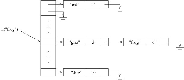
Now let’s consider how we would look up a key. First, we need to obtain the key’s hash code by calling its GetHashCode method. From the hash code, we use the division method to compute the table location where it belongs. We then search the linked list for that key.

Adding a key and a value is done similarly. We first look for the key as described above. If we find it, we either replace its KeyValuePair with a new one containing the new value, or we throw an exception, depending on how we want this method to behave. If we don’t find it, we add a new cell containing the given key and value to the beginning of the list we searched.

Note that looking up a key or adding a key and a value as described above can be implemented using either methods or indexers (.NET uses both). See the section, “Indexers” for details on how to implement an indexer.

Rehashing

In this section, we will show how to improve the performance of a hash table by adjusting the size of the array. In order to see how the array size impacts the performance, let’s suppose we are using an array with $ m $ locations, and that we are storing $ n $ keys in the hash table. In what follows, we will analyze the number of keys we will need to examine while searching for a particular key, k.

In the worst case, no matter how large the array is, it is possible that all of the keys map to the same array location, and therefore all end up in one long linked list. In such a case, we will need to examine all of the keys whenever we are looking for the last one in this list. However, the worst case is too pessimistic — if the hash function is implemented properly, it is reasonable to expect that something approaching a uniform random distribution will occur. We will therefore consider the number of keys we would expect to examine, assuming a uniform random distribution of keys throughout the table.

We’ll first consider the case in which k is not in the hash table. In this case, we will need to examine all of the keys in the linked list at the array location where k belongs. Because each of the $ n $ keys is equally likely to map to each of the $ m $ array locations, we would expect, on average, $ n / m $ keys to be mapped to the location where k belongs. Hence, in this case, we would expect to examine $ n / m $ keys, on average.

Now let’s consider the case in which k is in the hash table. In this case, we will examine the key k, plus all the keys that precede k in its linked list. The number of keys preceding k cannot be more than the total number of keys other than k in that linked list. Again, because each of the $ n - 1 $ keys other than k is equally likely to map to each of the $ m $ array locations, we would expect, on average, $ (n - 1) / m $ keys other than k to be in the same linked list as k. Thus, we can expect, on average, to examine no more than $ 1 +  (n - 1) / m $ keys when looking for a key that is present.

Notice that both of the values derived above decrease as $ m $ increases. Specifically, if $ m \geq n $, the expected number of examined keys on a failed lookup is no more than $ 1 $, and the expected number of examined keys on a successful lookup is less than $ 2 $. We can therefore expect to achieve very good performance if we keep the number of array locations at least as large as the number of keys.

We have already seen (e.g., in “Implementation of StringBuilders ”) how we can keep an array large enough by doubling its size whenever we need to. However, a hash table presents two unique challenges for this technique. First, as we observed in the previous section , we are most likely to get good performance from a hash table if the number of array locations is a prime number. However, doubling a prime number will never give us a prime number. The other challenge is due to the fact that when we change the size of the array, we consequently change the hash function, as the hash function uses the array size. As a result, the keys will need to go to different array locations in the new array.

In order to tackle the first challenge, recall that we presented an algorithm for finding all prime numbers less than a given n in “Finding Prime Numbers ”; however, this is a rather expensive way to find a prime number of an appropriate size. While there are more efficient algorithms, we really don’t need one. Suppose we start with an array size of $ 5 $ (there may be applications using many small hash tables — the .NET implementation starts with an array size of $ 3 $). $ 5 $ is larger than $ 2^2 = 4 $. If we double this value $ 28 $ times, we reach a value larger than $ 2^{30} $, which is larger than $ 1 $ billion. More importantly, this value is large enough that we can’t double it again, as an array in C# must contain fewer than $ 2^{31} $ locations. Hence, we need no more than $ 29 $ different array sizes. We can pre-compute these and hard-code them into our implementation; for example,

private int[] _tableSizes = 
{
    5, 11, 23, 47, 97, 197, 397, 797, 1597, 3203, 6421, 12853, 25717,
    51437, 102877, 205759, 411527, 823117, 1646237, 3292489, 6584983,
    13169977, 26339969, 52679969, 105359939, 210719881, 421439783,
    842879579, 1685759167 
}; 

Each of the values in the above array is a prime number, and each one after the first is slightly more than twice its predecessor. In order to make use of these values, we need a private field to store the index at which the current table size is stored in this array. We also need to keep track of the number of keys currently stored. As this information is useful to the user, a public int Count property would be appropriate. It can use the default implementation with a get accessor and a private set accessor.

One important difference between the reason for rehashing and the reason for creating a larger array for an implementation of a StringBuilder , stack , or queue is that rehashing is done simply for performance reasons - there is always room to put a new key and value into a hash table unless we have run out of memory. For this reason, it makes sense to handle rehashing after we have added the new key and value. This results in one extra linked-list insertion (i.e., updating two references) each time we rehash, but it simplifies the coding somewhat. Because rehashing is rarely done, this overhead is minimal, and seems to be a reasonable price to pay for simpler code.

Once a new key and value have been added, we first need to update the Count. We then need to check to see whether this number exceeds the current array size. As we do this, we should also make sure that the array size we are using is not the last array size in _tableSizes, because if it is, we can’t rehash. If both of these conditions hold, we need to rehash.

To begin rehashing, we copy the reference to the table into a local variable and increment the field giving our current index into _tableSizes. We then construct for the table field a new array whose size is given by the value at the new current index into _tableSizes. Note that it is important that the local variable is used to refer to the old table, and that the field is used to refer to the new table, as the hash function uses the field to obtain the array size.

We then need to move all keys and values from the old table to the new one. As we do this, we will need to re-compute the hash function for each key, as the hash function has now changed. We therefore need two nested loops. The outer loop iterates through the locations in the old table, and the inner loop iterates through the linked list at that location. On each iteration of the inner loop:

1. Use a local variable to save another reference to the current cell in the linked list at the current table location.
2. Advance to the next cell in the list.
3. Using the hash function, compute the new array location of the key in the cell that was saved in step 1.
4. Insert this cell into the beginning of the linked list at the new array location in the new table.

Memoization

We we will now present an example of a common technique involving dictionaries. Consider the following variation of the 2-player game, Nim. The board consists of a number of stones arranged into several piles. Associated with each nonempty pile is a limit, which is a positive integer no greater than the number of stones on that pile (the limit for an empty pile is always 0). Players alternate taking stones according to the following rules:

• On each turn, the player must take some number of stones from a single pile.
• The number of stones taken must be at least 1, but no more than the current limit for that pile.
• Taking n stones from a pile changes the limit for that pile to 2n. (If this limit is more than the number of stones remaining on that pile, the new limit is the number of stones remaining.)

The player taking the last stone wins. Note that by the rules of the game, there will always be a winner — a draw is impossible.

For example, suppose we start a game with three piles, each containing 10 stones with a limit of 9. We will denote this board position as (10/9; 10/9; 10/9). If Player 1 removes two stones from Pile 1, the resulting position is (8/4; 10/9; 10/9). Note that because 2 stones were removed from Pile 1, its new limit is 2 x 2 = 4. If Player 2 now removes 4 stones from Pile 2, the resulting position is (8/4; 6/6; 10/9). Note that because 4 stones were removed, the new limit for Pile 2 would become 2 x 4 = 8; however, because only 6 stones remain, the new limit is 6. Play then continues until a player wins by taking all remaining stones.

Let us define a winning play as any play giving a position from which there is no winning play. Thus, if we make a winning play, there are two possible cases. In the first case, there are no winning plays from the resulting position because there are no legal plays. This means we just took the last stone and won the game. In the other case, there are legal plays, but none is a winning play. Our opponent must make one of these plays. Because it isn’t a winning play, there must be a winning play from the resulting position. Therefore, an optimal strategy is to make a winning play whenever one exists. Because of the way a winning play is defined, if a winning play exists, following this strategy will enable us to continue to make winning plays until we eventually win the game. If no winning play exists, we just have to make some play and hope that our opponent blunders by making a play that is not a winning play. If that happens, a winning play will be available, and our strategy leads us to a win.

Consider the following examples:

• Example 1: (1/1; 0/0). Taking one stone from Pile 1 is a winning play because there is no legal play from the resulting position; hence, there can be no winning play from it.
• Example 2: (1/1; 1/1). There is no winning play from this position because both legal plays give essentially the position from Example 1, from which there is a winning play.
• Example 3: (2/2; 1/1). Taking one stone from Pile 1 is a winning play because it leads to (1/1; 1/1), from which there is no winning play, as shown in Example 2.

Given enough stones and piles, finding a winning play or determining that there is none is challenging. In order to develop a search algorithm somewhat similar to the one described in “Tries in Word Games” , we can define the following tree:

• The root is the current board position.
• The children of a node are all the positions that can be reached by making legal plays.

Thus, the tree defined by (2/2; 2/2) is as follows:

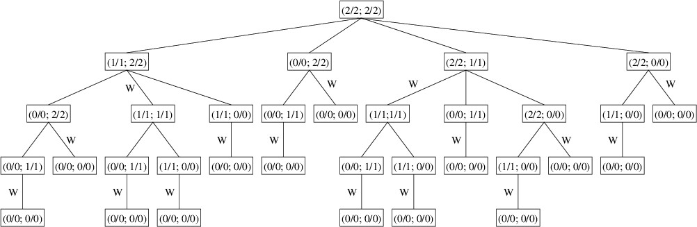
The winning plays have each been marked with a ‘W’ in the above tree. As in “Tries in Word Games” , this tree is not a data structure, but simply a mental guide to building a search algorithm. Specifically, we can find a winning play (or determine whether there is none) by traversing the tree in the following way:

• For each legal play p from the given position:
  • Form the board position that results from making this play (this position is a child).
  • Recursively find a winning play from this new position.
  • If there was no winning play returned (i.e., it was null), return p, as it’s a winning play.
• If we get to this point we’ve examined all the plays, and none of them is winning; hence we return null.

Note that the above algorithm may not examine all the nodes in the tree because once it finds a winning play, it returns it immediately without needing to examine any more children. For example, when processing the children of the node (1/1; 2/2), it finds that from its second child, (1/1; 1/1), there is no winning play; hence, it immediately returns the play that removes one stone from Pile 2 without even looking at the third child, (1/1; 0/0). Even so, because the size of the tree grows exponentially as the number of stones increases, once the number of stones reaches about 25, the time needed for the algorithm becomes unacceptable.

Notice that several of the nodes in the tree occur multiple times. For example, (1/1; 1/1) occurs twice and (1/1; 0/0) occurs five times. For a large tree, the number of duplicate nodes in the tree increases dramatically. The only thing that determines the presence of a winning move is the board position; hence, once we have a winning move (or know that none exists) for a given position, it will be the same wherever this position may occur in the tree. We can therefore save a great deal of time by saving the winning move for any position we examine. Then whenever we need to examine a position, we first check to see if we’ve already processed it — if so, we just use the result we obtained earlier rather than processing it again. Because processing it again may involve searching a large tree, the savings in time might be huge.

The technique outlined in the above paragraph is known as memoization (not to be confused with memorization) — we make a memo of the results we compute so that we can look them up again later if we need them. A dictionary whose keys are board positions and whose values are plays is an ideal data structure for augmenting the above search with memoization. As the first step, before we look at any plays from the given board position, we look up the position in the dictionary. If we find it, we immediately return the play associated with it. Otherwise, we continue the algorithm as before, but prior to returning a play (even if it is null), we save that play in the dictionary with the given board position as its key. This memoization will allow us to analyze board positions containing many more stones.

To implement the above strategy, we need to define two types - one to represent a board position and one to represent a play. The type representing a play needs to be a class so that we can use null to indicate that there is no winning play. The type representing a board position can be either a class or a structure. Because the dictionary needs to be able to compare instances of this type for equality in order be able to find keys, its definition will need to re-define the equality comparisons. Consequently, we need to redefine the hash code computation to be consistent with the equality comparison. The next two sections will examine these topics.

Equality in C#

Continuing our discussion from the previous section , we want to define a type that represents a Nim board. Furthermore, we need to be able to compare instances of this type for equality. Before we can address how this can be done, we first need to take a careful look at how C# handles equality. In what follows, we will discuss how C# handles the == operator, the non-static Equals method, and two static methods for determining equality. We will then show how the comparison can be defined so that all of these mechanisms behave in a consistent way.

We first consider the == operator. The behavior of this operator is determined by the compile-time types of its operands. This is determined by the declared types of variables, the declared return types of methods or properties, and the rules for evaluating expressions. Thus, for example, if we have a statement

object x = "abc";

the compile-time type of x is object, even though it actually refers to a string.

For pre-defined value types , == evaluates to true if its operands contain the same values. Because enumerations are represented as numeric types such as int or byte, this rule applies to them as well. For user-defined structures, == is undefined unless the structure definition explicitly defines the == and != operators. We will show how this can be done below.

By default, when == is applied to reference types, it evaluates to true when the two operands refer to the same object (i.e., they refer to the same memory location). A class may override this behavior by explicitly defining the == and != operators. For example, the string class defines the == operator to evaluate to true if the given strings are the same length and contain the same sequence of characters.

Let’s consider an example that illustrates the rules for reference types:

string a = "abc";
string b = "0abc".Substring(1);
object x = a;
object y = b;
bool comp1 = a == b;
bool comp2 = x == y;

The first two lines assign to a and b the same sequence of characters; however, because the strings are computed differently, they are different objects. The next two lines copy the reference in a to x and the reference in b to y. Thus, at this point, all four variables refer to a string “abc”; however, a and x refer to a different object than do b and y. The fifth line compares a and b for equality using ==. The compile-time types of a and b are both string; hence, these variables are compared using the rules for comparing strings. Because they refer to strings of the same length and containing the same sequence of characters, comp1 is assigned true. The behavior of the last line is determined by the compile-time types of x and y. These types are both object, which defines the default behavior of this operator for reference types. Thus, the comparison determines whether the two variables refer to the same object. Because they do not, comp2 is assigned false.

Now let’s consider the non-static Equals method. The biggest difference between this method and the == operator is that the behavior of x.Equals(y) is determined by the run-time type of x. This is determined by the actual type of the object, independent of how any variables or return types are declared.

By default, if x is a value type and y can be treated as having the same type, then x.Equals(y) returns true if x and y have the same value (if y can’t be treated as having the same type as x, then this method returns false). Thus, for pre-defined value types, the behavior is the same as for == once the types are determined (provided the types are consistent). However, the Equals method is always defined, whereas the == operator may not be. Furthermore, structures may override this method to change this behavior — we will show how to do this below.

By default, if x is a reference type, x.Equals(y) returns true if x and y refer to the same object. Hence, this behavior is the same as for == once the types are determined (except that if x is null, x.Equals(y) will throw a NullReferenceException, whereas x == y will not). However, classes may override this method to change this behavior. For example, the string class overrides this method to return true if y is a string of the same length and contains the same sequence of characters as x.

Let’s now continue the above example by adding the following lines:

bool comp3 = a.Equals(b);
bool comp4 = a.Equals(x);
bool comp5 = x.Equals(a);
bool comp6 = x.Equals(y);

These all evaluate to true for one simple reason — the behavior is determined by the run-time type of a in the case of the first two lines, or of x in the case of the last two lines. Because these types are both string, the objects are compared as strings.

The object class defines, in addition to the Equals method described above, two public static methods, which are in turn inherited by every type in C#:

• bool Equals(object x, object y): The main purpose of this method is to avoid the NullReferenceException that is thrown by x.Equals(y) when x is null. If neither x nor y is null, this method simply returns the value of x.Equals(y). Otherwise, it will return true if both x and y are null, or false if only one is null. User-defined types cannot override this method, but because it calls the non-static Equals method, which they can override, they can affect its behavior indirectly.
• bool ReferenceEquals(object x, object y): This method returns true if x and y refer to the same object or are both null. If either x or y is a value type, it will return false. User-defined types cannot override this method.

Finally, there is nothing to prevent user-defined types from including their own Equals methods with different parameter lists. In fact, the string class includes definitions of the following public methods:

• bool Equals(string s): This method actually does the same thing as the non-static Equals method defined in the object class, but is slightly more efficient because less run-time type checking needs to be done. This is the method that is called in the computation of comp3 in the above example.
• static bool Equals(string x, string y): This method does the same thing as the static Equals method defined in the object class, but again is slightly more efficient because less run-time type checking needs to be done.

All of this can be rather daunting at first. Fortunately, in most cases these comparisons end up working the way we expect them to. The main thing we want to focus on here is how to define equality properly in a user-defined type.

Let’s start with the == operator. This is one of several operators that may be defined within class and structure definitions. If we are defining a class called SomeType, we can include a definition of the == operator as follows:

public static bool operator ==(SomeType? x, SomeType? y)
{
    // Definition of the behavior of ==
}

If SomeType is a structure, the definition is similar, but we wouldn’t define the parameters to be nullable. Note the resemblance to the definition of a static method. Even though we define it using the syntax for a method definition, we still use it as we typically use the == operator; e.g.,

if (a == b)
{
    . . .
}

If SomeType is a class and a and b are both of either type SomeType or type SomeType?, the above definition will be called using a as the parameter x and b as the parameter y.

Within the operator definition, if it is within a class definition, the first thing we need to do is to handle the cases in which one or both parameters are null. We don’t need to do this for a structure definition because value types can’t be null, but if we omit this part for a reference type, comparing a variable or expression of this type to null will most likely result in a NullReferenceException. We need to be a bit careful here, because if we use == to compare one of the parameters to null it will be a recursive call — infinite recursion, in fact. Furthermore, using x.Equals(null) is always a bad idea, as if x does, in fact, equal null, this will throw a NullReferenceException. We therefore need to use one of the static methods, Equals or ReferenceEquals:

public static bool operator ==(SomeType? x, SomeType? y)
{
    if (Equals(x, null))
    {
         return (Equals(y, null));
    }
    else if (Equals(y, null))
    {
        return false;
    }
    else
    {
        // Code to determine if x == y
    }
}

Note that because all three calls to Equals have null as a parameter, these calls won’t result in calling the Equals method that we will override below.

Whenever we define the == operator, C# requires that we also define the != operator. In virtually all cases, what we want this operator to do is to return the negation of what the == operator does; thus, if SomeType is a class, we define:

public static bool operator !=(SomeType? x, SomeType? y)
{
    return !(x == y);
}

If SomeType is a structure, we use the same definition, without making the parameters nullable.

We now turn to the (non-static) Equals method. This is defined in the object class to be a virtual method, meaning that sub-types are allowed to override its behavior. Because every type in C# is a subtype of object, this method is present in every type, and it can be overridden by any class or structure.

We override this method as follows:

public override bool Equals(object? obj)
{
    // Definition of the behavior of Equals
}

For the body of the method, we first need to take care of the fact that the parameter is of type object; hence, it may not even have the same type as what we want to compare it to. If this is the case, we need to return false. Otherwise, in order to ensure consistency between this method and the == operator, we can do the actual comparison using the == operator. If we are defining a class SomeType, we can accomplish all of this as follows:

public override bool Equals(object? obj)
{
    return obj as SomeType == this;
}

The as keyword casts obj to SomeType if possible; however, if obj cannot be cast to SomeType, the as expression evaluates to null (or in general, the default value for SomeType). Because this cannot be null, false will always be returned if obj cannot be cast to SomeType.

If SomeType is a structure, the above won’t work because this may be the default value for SomeType. In this case, we need somewhat more complicated code:

public override bool Equals(object? obj)
{
    if (obj is SomeType x)
    {
        return this == x;
    }
    else
    {
        return false;
    }
}

This code uses the is keyword, which is similar to as in that it tries to cast obj to SomeType. However, if the cast is allowed, it places the result in the SomeType variable x and evaluates to true; otherwise, it assigns to x the default value of SomeType and evaluates to false.

The above definitions give a template for defining the == and != operators and the non-static Equals method for most types that we would want to compare for equality. All we need to do to complete the definitions is to replace the name SomeType, wherever it occurs, with the name of the type we are defining, and to fill in the hole left in the definition of the == operator. It is here where we actually define how the comparison is to be made.

Suppose, for example, that we want to define a class to represent a Nim board position (see the previous section ). This class will need to have two private fields: an int[ ] storing the number of stones on each pile and an int[ ] storing the limit for each pile. These two arrays should be non-null and have the same length, but this should be enforced by the constructor. By default, two instances of a class are considered to be equal (by either the == operator or the non-static Equals method) if they are the same object. This is too strong for our purposes; instead, two instances x and y of the board position class should be considered equal if

• Their arrays giving the number of stones on each pile have the same length; and
• For each index i into the arrays giving the number of stones on each pile, the elements at location i of these arrays have the same value, and the elements at location i of the arrays giving the limit for each pile have the same value.

Code to make this determination and return the result can be inserted into the above template defining of the == operator, and the other two templates can be customized to refer to this type.

Any class that redefines equality should also redefine the hash code computation to be consistent with the equality definition. We will show how to do this in the next section.

Hash Codes

Whenever equality is redefined for a type, the hash code computation for that type needs to be redefined in a consistent way. This is done by overriding that type’s GetHashCode method. In order for hashing to be implemented correctly and efficiently, this method should satisfy the following goals:

• Equal keys must have the same hash code. This is necessary in order for the Dictionary<TKey, TValue> class to be able to find a given key that it has stored. On the other hand, because the number of possible keys is usually larger than the number of possible hash codes, unequal keys are also allowed to have the same hash code.
• The computation should be done quickly.
• Hash codes should be uniformly distributed even if the keys are not.

The last goal above may seem rather daunting, particularly in light of our desire for a quick computation. In fact, it is impossible to guarantee in general — provided there are more than $ 2^{32}(k - 1) $ possible keys from which to choose, no matter how the hash code computation is implemented, we can always find at least $ k $ keys with the same hash code. However, this is a problem that has been studied a great deal, and several techniques have been developed that are effective in practice. We will caution, however, that not every technique that looks like it should be effective actually is in practice. It is best to use techniques that have been demonstrated to be effective in a wide variety of applications. We will examine one of these techniques in what follows.

A guiding principle in developing hashing techniques is to use all information available in the key. By using all the information, we will be sure to use the information that distinguishes this key from other keys. This information includes not just the values of the individual parts of the the key, but also the order in which they occur, provided this order is significant in distinguishing unequal keys. For example, the strings, “being” and “begin” contain the same letters, but are different because the letters occur in a different order.

One specific technique initializes the hash code to 0, then processes the key one component at a time. These components may be bytes, characters, or other parts no larger than 32 bits each. For example, for the Nim board positions discussed in “Memoization” , the components would be the number of stones on each pile, the limit for each pile, and the total number of piles (to distinguish between a board ending with empty piles and a board with fewer piles). For each component, it does the following:

• Multiply the hash code by some fixed odd integer.
• Add the current component to the hash code.

Due to the repeated multiplications, the above computation will often overflow an int. This is not a problem — the remaining bits are sufficient for the hash code.

In order to understand this computation a little better, let’s first ignore the effect of this overflow. We’ll denote the fixed odd integer by $ x $, and the components of the key as $ k_1, \dots, k_n $. Then this is the result of the computation:

Because the above is a polynomial, this hashing scheme is called polynomial hashing. While the computation itself is efficient, performing just a couple of arithmetic operations on each component, the result is to multiply each component by a unique value ( $ x^i $ for some $ i $) depending on its position within the key.

Now let’s consider the effect of overflow on the above polynomial. What this does is to keep only the low-order 32 bits of the value of the polynomial. Looking at it another way, we end up multiplying $ k_i $ by only the low-order 32 bits of $ x^{n-i} $. This helps to explain why $ x $ is an odd number — raising an even number to the $ i $th power forms a number ending in $ i $ 0s in binary. Thus, if there are more than 32 components in the key, all but the last 32 will be multiplied by $ 0 $, and hence, ignored.

There are other potential problems with using certain odd numbers for $ x $. For example, we wouldn’t want to use $ 1 $, because that would result in simply adding all the components together, and we would lose any information regarding their positions within the key. Using $ -1 $ would be almost as bad, as we would multiply all components in odd positions by $ -1 $ and all components in even positions by $ 1 $. The effect of overflow can cause similar behavior; for example, if we place $ 2^{31} - 1 $ in an int variable and square it, the overflow causes the result to be 1. Successive powers will then alternate between $ 2^{31} - 1 $ and $ 1 $.

It turns out that this cyclic behavior occurs no matter what odd number we use for $ x $. However, in most cases the cycle is long enough that keys of a reasonable size will have each component multiplied by a unique value. The only odd numbers that result in short cycles are those that are adjacent to a multiple of a large power of $ 2 $ (note that $ 0 $ is a multiple of any integer).

The other potential problem occurs when we are hashing fairly short keys. In such cases, if $ x $ is also small enough, the values computed will all be much smaller than the maximum possible integer value $ (2^{31} - 1) $. As a result, we will not have a uniform distribution of values. We therefore want to avoid making $ x $ too small.

Putting all this together, choosing $ x $ to be an odd number between $ 30 $ and $ 40 $ works pretty well. These values are large enough so that seven key components will usually overflow an int. Furthermore, they all have a cycle length greater than $ 100 $ million.

We should always save the hash code in a private field after we compute it so that subsequent requests for the same hash code don’t result in repeating the computation. This can be done in either of two ways. One way is to compute it in an eager fashion by doing it in the constructor. When doing it this way, the GetHashCode method simply needs to return the value of the private field. While this is often the easiest way, it sometimes results in computing a hash code that we end up not using. The alternative is to compute it in a lazy fashion. This requires an extra private field of type bool. This field is used to indicate whether the hash code has been computed yet or not. With this approach, the GetHashCode method first checks this field to see if the hash code has been computed. If not, it computes the hash code and saves it in its field. In either case, it then returns the value of the hash code field.