Introduction to Graphs

There are two kinds of graphs: undirected and directed. An undirected graph consists of:

• a finite set of nodes; and
• a finite set of edges, which are 2-element subsets of the nodes.

The fact that edges are 2-element sets means that the nodes that comprise an edge must be distinct. Furthermore, within a set, there is no notion of a “first” element or a “second” element — there are just two elements. Thus, an edge expresses some symmetric relationship between two nodes; i.e., if $ \{u, v\} $ is an edge then node $ u $ is adjacent to node $ v $, and node $ v $ is adjacent to node $ u $. We also might associate some data, such as a label or a length, with an edge.

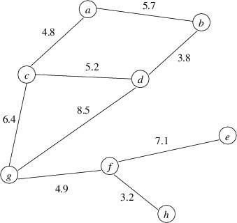
We can think of an edge as “connecting” the two nodes that comprise it. We can then draw an undirected graph using circles for the nodes and lines connecting two distinct nodes for the edges. Following is an example of an undirected graph with numeric values associated with the edges:

A directed graph is similar to an undirected graph, but the edges are ordered pairs of distinct nodes rather than 2-element sets. Within an ordered pair, there is a first element and a second element. We call the first node of an edge its source and the second node its destination. Thus, an edge in a directed graph expresses an asymmetric relationship between two nodes; i.e., if $ (u, v) $ is an edge, then $ v $ is adjacent to $ u $, but $ u $ is not adjacent to $ v $ unless $ (v, u) $ is also an edge in the graph. As with undirected graphs, we might associate data with an edge in a directed graph.

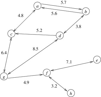
We can draw directed graphs like we draw undirected graphs, except that we use an arrow to distinguish between the source and the destination of an edge. Specifically, the arrows point from the source to the destination. If we have edges $ (u, v) $ and $ (v, u) $, and if these edges have the same data associated with them, we might simplify the drawing by using a single line with arrows in both directions. Following is an example of a directed graph with numeric values associated with the edges:

This DLL contains the definition of a namespace Ksu.Cis300.Graphs containing a class DirectedGraph<TNode, TEdgeData> and a readonly structure Edge<TNode, TEdgeData>. It requires a DLL for Ksu.Cis300.LinkedListLibrary within the same directory. The class DirectedGraph<TNode, TEdgeData> implements a directed graph whose nodes are of type TNode, which must be non-nullable. The edges each store a data item of type TEdgeData, which may be any type. These edges can be represented using instances of the Edge<TNode, TEdgeData> structure. We also can use the DirectedGraph<TNode, TEdgeData> class to represent undirected graphs — we simply make sure that whenever there is an edge $ (u, v) $, there is also an edge $ (v, u) $ containing the same data.

The Edge<TNode, TEdgeData> structure contains the following public members:

• Edge(TNode source, TNode dest, TEdgeData data): This constructor constructs an edge leading from source to dest and having data as its data item.
• TNode Source: This property gets the source node for the edge.
• TNode Destination: This property gets the destination node for the edge.
• TEdgeData Data: This property gets the data associated with the edge.

The DirectedGraph<TNode, TEdgeData> class contains the following public members:

• DirectedGraph(): This constructor constructs a directed graph with no nodes or edges.
• void AddNode(TNode node): This method adds the given node to the graph. If this node already is in the graph, it throws an ArgumentException. If node is null, it throws an ArgumentNullException.
• void AddEdge(TNode source, TNode dest, TEdgeData value): This method adds a new edge from source to dest, with value as its associated value. If either source or dest is not already in the graph, it is automatically added. If source and dest are the same node, or if there is already an edge from source to dest, it throws an ArgumentException. If either source or dest is null, it throws an ArgumentNullException.
• bool TryGetEdge(TNode source, TNode dest, out TEdgeData? value): This method tries to get the value associated with the edge from source to dest. If this edge exists, it sets value to the value associated with this edge and returns true; otherwise, it sets value to the default value for the TEdge type and returns false.
• int NodeCount: This property gets the number of nodes in the graph.
• int EdgeCount: This property gets the number of edges in the graph.
• bool ContainsNode(TNode node): This method returns whether the graph contains the given node. If node is null, it throws an ArgumentNullException.
• bool ContainsEdge(TNode source, TNode dest): This method returns whether the graph contains an edge from source to dest.
• IEnumerable<TNode> Nodes: This property gets an enumerable collection of the nodes in the graph.
• IEnumerable<Edge<TNode, TEdgeData>> OutgoingEdges(TNode source): This method gets an enumerable collection of the outgoing edges from the given node. If source is not a node in the graph, it throws an ArgumentException. If source is null, it throws an ArgumentNullException. Otherwise, each edge in the collection returned is represented by an Edge<TNode, TEdgeData>

This implementation is somewhat limited in its utility, as nodes or edges cannot be removed, and values associated with edges cannot be changed. However, it will be sufficient for our purposes. We will examine its implementation details in a later section . For now, we will examine how it can be used.

Building a graph is straightforward using the constructor and the AddNode and/or AddEdge methods. Note that because the AddEdge method will automatically add given nodes that are not already in the graph, the AddNode method is only needed when we need to add a node that may have no incoming or outgoing edges.

For many graph algorithms, we need to process all of the edges in some way. Often the order in which we process them is important, but not in all cases. If we simply need to process all of the edges in some order we can use foreach loops with the last two members listed above to accomplish this:

• For each node in the graph:
  • For each outgoing edge from that node:
    • Process this edge.

Shortest Paths

In this section, we will consider a common graph problem — that of finding a shortest path from a node u to a node v in a directed graph. We will assume that each edge contains as its data a nonnegative number. This number may represent a physical distance or some other cost, but for simplicity, we will refer to this value as the length of the edge. We can then define the length of a path to be the sum of the lengths of all the edges along that path. A shortest path from u to v is then a path from u to v with minimum length. Thus, for example, the shortest path from a to h in the graph below is a-c-g-f-h, and its length is 4.8 + 6.4 + 4.9 + 3.2 = 19.3.

The biggest challenge in finding an algorithm for this problem is that the number of paths in a graph can be huge, even for relatively small graphs. For example, a directed graph with 15 nodes might contain almost 17 billion paths from a node u to a node v. Clearly, an algorithm that simply checks all paths would be impractical for solving a problem such as finding the shortest route between two given locations in North America. In what follows, we will present a much more efficient algorithm due to Edsger W. Dijkstra.

First, it helps to realize that when we are looking for a shortest path from u to v, we are likely to find other shortest paths along the way. Specifically, if node w is on the shortest path from u to v, then taking that same path but stopping at w gives us a shortest path from u to w. Returning to the above example, the shortest path from a to h also gives us shortest paths from a to each of the nodes c, g, and f. For this reason, we will generalize the problem to that of finding the shortest paths from a given node u to each of the nodes in the graph. This problem is known as the single-source shortest paths problem. This problem is a bit easier to think about because we can use shortest path information that we have already computed to find additional shortest path information. Then once we have an algorithm for this problem, we can easily modify it so that as soon as it finds the shortest path to our actual goal node v, we terminate it.

Dijkstra’s algorithm progresses by finding a shortest path to one node at a time. Let S denote the set of nodes to which it has found a shortest path. Initially, S will contain only u, as the shortest path from u to u is the empty path. At each step, it finds a shortest path that begins at u and ends at a node outside of S. Let’s call the last node in this path x. Certainly, if this path to x is the shortest to any node outside of S, it is also the shortest to x. The algorithm therefore adds x to S, and continues to the next step.

What makes Dijkstra’s algorithm efficient is the way in which it finds each of the paths described above. Recall that each edge has a nonnegative length. Hence, once a given path reaches some node outside of S, we cannot make the path any shorter by extending it further. We therefore only need to consider paths that remain in S until the last edge, which goes from a node in S to a node outside of S. We will refer to such edges as eligible. We are therefore looking for a shortest path whose last edge is eligible.

Suppose (w, x) is an eligible edge; i.e., w is in S, but x is not. Because w is in S, we know the length of the shortest path to w. The length of a shortest path ending in (w, x) is simply the length of the shortest path to w, plus the length of (w, x).

Let us therefore assign to each eligible edge (w, x) a priority equal to the length of the shortest path to w, plus the length of (w, x). A shortest path ending in an eligible edge therefore has a length equal to the minimum priority of any eligible edge. Furthermore, if the eligible edge with minimum priority is (w, x), then the shortest path to x is the shortest path to w, followed by (w, x).

We can efficiently find an eligible edge with minimum priority if we store all eligible edges in a MinPriorityQueue<TEdgeData, Edge<TNode, TEdgeData>>. Note however, that when we include x in S as a result of removing (w, x) from the queue, it will cause any other eligible edges leading to x to become ineligible, as x will no longer be outside of S. Because removing these edges from the min-priority queue is difficult, we will simply leave them in the queue, and discard them whenever they have minimum priority. This min-priority queue will therefore contain all eligible edges, plus some edges whose endpoints are both in S.

We also need a data structure to keep track of the shortest paths we have found. A convenient way to do this is, for each node to which we have found a shortest path, to keep track of this node’s predecessor on this path. This will allow us to retrieve a shortest path to a node v by starting at v and tracing the path backwards using the predecessor of each node until we reach u. A Dictionary<TNode, TNode> is an ideal choice for this data structure. The keys in the dictionary will be the nodes in S, and the value associated with a key will be that key’s predecessor on a shortest path. For node u, which is in S but has no predecessor on its shortest path, we can associate a value of u itself.

The algorithm begins by adding the key u with the value u to a new dictionary. Because all of the outgoing edges from u are now eligible, it then places each of these edges into the min-priority queue. Because u is the source node of each of these edges, and the shortest path from u to u has length 0, the priority of each of these edges will simply be its length.

Once the above initialization is done, the algorithm enters a loop that iterates as long as the min-priority queue is nonempty. An iteration begins by obtaining the minimum priority p from the min-priority queue, then removing an edge (w, x) with minimum priority. If x is a key in the dictionary, we can ignore this edge and go on to the next iteration. Otherwise, we add to the dictionary the key x with a value of w. Because we now have a shortest path to x, there may be more eligible edges that we need to add to the min-priority queue. These edges will be edges from x that lead to nodes that are not keys in the dictionary; however, because the min-priority queue can contain edges to nodes that are already keys, we can simply add all outgoing edges from x. Because the length of the shortest path to x is p, the priority of each of these outgoing edges is p plus the length of the outgoing edge.

Note that an edge is added to the min-priority queue only when its source is added as a key to the dictionary. Because we can only add a key once, each edge is added to the min-priority queue at most once. Because each iteration removes an edge from the min-priority queue, the min-priority queue must eventually become empty, causing the loop to terminate. When the min-priority queue becomes empty, there can be no eligible edges; hence, when the loop terminates, the algorithm has found a shortest path to every reachable node.

We can now modify the above algorithm so that it finds a shortest path from u to a given node v. Each time we add a new key to the dictionary, we check to see if this key is v; if so, we return the dictionary immediately. We might also want to return this path’s length, which is the priority of the edge leading to v. In this case, we could return the dictionary as an out parameter. Doing this would allow us to return a special value (e.g., a negative number) if we get through the loop without adding v, as this would indicate that v is unreachable. This modified algorithm is therefore as follows:

• Construct a new dictionary and a new min-priority queue.
• Add to the dictionary the key u with value u.
• If u = v, return 0.
• For each outgoing edge (u, w) from u:
  • Add (u, w) to the min-priority queue with a priority of the length of this edge.
• While the min-priority queue is nonempty:
  • Get the minimum priority p from the min-priority queue.
  • Remove an edge (w, x) with minimum priority from the min-priority queue.
  • If x is not a key in the dictionary:
    • Add to the dictionary the key x with a value of w.
    • If x = v, return p.
    • For each outgoing edge (x, y) from x:
      • Add (x, y) to the min-priority queue with priority p plus the length of (x, y).
• Return a negative value.

The above algorithm computes all of the path information we need, but we still need to extract from the dictionary the shortest path from u to v. Because the value for each key is that key’s predecessor, we can walk backward through this path, starting with v. To get the path in the proper order, we can push the nodes onto a stack; then we can remove them in the proper order. Thus, we can extract the shortest path as follows:

• Construct a new stack.
• Set the current node to v.
• While the current node is not u:
  • Push the current node onto the stack.
  • Set the current node to its value in the dictionary.
• Process u.
• While the stack is not empty:
  • Pop the top node from the stack and process it.

Unweighted Shortest Paths

In some shortest path problems, all edges have the same length. For example, we may be trying to find the shortest path out of a maze. Each cell in the maze is a node, and an edge connects two nodes if we can move between them in a single step. In this problem, we simply want to minimize the number of edges in a path to an exit. We therefore say that the edges are unweighted — they contain no explicit length information, and the length of each edge is considered to be $ 1 $.

We could of course apply Dijkstra’s algorithm to this problem, using $ 1 $ as the length of each edge. However, if analyze what this algorithm does in this case, we find that we can optimize it to achieve significantly better performance.

The optimization revolves around the use of the min-priority queue. Note that Dijkstra’s algorithm first adds all outgoing edges from the start node u to the min-priority queue, using their lengths as their priorities. For unweighted edges, each of these priorities will be $ 1 $. As the algorithm progresses it retrieves the minimum priority and removes an edge having this priority. If it adds any new edges before removing the next edge, they will all have a priority $ 1 $ greater than the priority of the edge just removed.

We claim that this behavior causes the priorities in the min-priority queue to differ by no more than $ 1 $. To see this, we will show that we can never reach a point where we change the maximum difference in priorities from at most $ 1 $ to more than $ 1 $. First observe that when the outgoing edges from u are added, the priorities all differ by $ 0 \leq 1 $. Removing an edge can’t increase the difference in the priorities stored. Suppose the edge we remove has priority $ p $. Assuming we have not yet achieved a priority difference greater than $ 1 $, any priorities remaining in the min-priority queue must be either $ p $ or $ p + 1 $. Any edges we add before removing the next edge have priority $ p + 1 $. Hence, the priority difference remains no more than $ 1 $. Because we have covered all changes to the priority queue, we can never cause the priority difference to exceed $ 1 $.

Based on the above claim, we can now claim that whenever an edge is added, its priority is the largest of any in the min-priority queue. This is certainly true when we add the outgoing edges from u, as all these edges have the same priority. Furthermore, whenever we remove an edge with priority $ p $, any edges we subsequently add have priority $ p + 1 $, which must be the maximum priority in the min-priority queue.

As a result of this behavior, we can replace the min-priority queue with an ordinary FIFO queue , ignoring any priorities. For a graph with unweighted edges, the behavior of the algorithm will be the same. Because accessing a FIFO queue is more efficient than accessing a min-priority queue, the resulting algorithm, known as breadth-first search, is also more efficient.

Implementing a Graph

Traditionally, there are two main techniques for implementing a graph. Each of these techniques has advantages and disadvantages, depending on the characteristics of the graph. In this section, we describe the implementation of the DirectedGraph<TNode, TEdgeData> class from Ksu.Cis300.Graphs.dll . This implementation borrows from both traditional techniques to obtain an implementation that provides good performance for any graph. In what follows, we will first describe the two traditional techniques and discuss the strengths and weaknesses of each. We will then outline the implementation of DirectedGraph<TNode, TEdgeData>.

The first traditional technique is to use what we call an adjacency matrix. This matrix is an $ n \times n $ boolean array, where $ n $ is the number of nodes in the graph. In this implementation, each node is represented by an int value $ i $, where $ 0 \leq i \lt n $. The value at row $ i $ and column $ j $ will be true if there is an edge from node $ i $ to node $ j $.

The main advantage to this technique is that we can very quickly determine whether an edge exists — we only need to look up one element in an array. There are several disadvantages, however. First, we are forced to use a specific range of int values as the nodes. If we wish to have a generic node type, we need an additional data structure (such as a Dictionary<TNode, int>) to map each node to its int representation. It also fails to provide a way to associate a value with an edge; hence, we would need an additional data structure (such as a TEdgeData[int, int]) to store this information.

Perhaps the most serious shortcoming for the adjacency matrix, however, is that if the graph contains a large number of nodes, but relatively few edges, it wastes a huge amount of space. Suppose, for example, that we have a graph representing street information, and suppose there are about one million nodes in this graph. We might expect the graph to contain around three million edges. However, an adjacency matrix would require one trillion entries, almost all of which will be false. Similarly, finding the edges from a given node would require examining an entire row of a million elements to find the three or four outgoing edges from that node.

The other traditional technique involves using what we call adjacency lists. An adjacency list is simply a linked list containing descriptions of the outgoing edges from a single node. These lists are traditionally grouped together in an array of size $ n $, where $ n $ is again the number of nodes in the graph. As with the adjacency matrix technique, the nodes must be nonnegative ints less than $ n $. The linked list at location $ i $ of the array then contains the descriptions of the outgoing edges from node $ i $.

One advantage to this technique is that the amount of space it uses is proportional to the size of the graph (i.e., the number of nodes plus the number of edges). Furthermore, obtaining the outgoing edges from a given node simply requires traversing the linked list containing the descriptions of these edges. Note also that we can store the data associated with an edge within the linked list cell describing that edge. However, this technique still requires some modification if we wish to use a generic node type. A more serious weakness, though, is that in order to determine if a given edge exists, we must search through potentially all of the outgoing edges from a given node. If the number of edges is large in comparison to the number of nodes, this search can be expensive.

As we mentioned above, our implementation of DirectedGraph<TNode, TEdgeData> borrows from both of these traditional techniques. We start by modifying the adjacency lists technique to use a Dictionary<TNode, LinkedListCell<TNode>?> instead of an array of linked lists. Thus, we can accommodate a generic node type while maintaining efficient access to the adjacency lists. While a dictionary lookup is not quite as efficient as an array lookup, a dictionary would provide the most efficient way of mapping nodes of a generic type to int array indices. Using a dictionary instead of an array eliminates the need to do a subsequent array lookup. The linked list associated with a given node in this dictionary will then contain the destination node of each outgoing edge from the given node.

In addition to this dictionary, we use a Dictionary<(TNode, TNode), TEdgeData> to facilitate efficient edge lookups. The notation (T1, T2) defines a tuple, which is an ordered pair of elements, the first of type T1, and the second of type T2. Elements of this type are described with similar notation, (x, y), where x is of type T1 and y is of type T2. These elements can be accessed using the public properties Item1 and Item2. In general, longer tuples can be defined similarly.

This second dictionary essentially fills the role of an adjacency matrix, while accommodating a generic node type and using space more efficiently. Specifically, a tuple whose Item1 is u and whose Item2 is v will be a key in this dictionary if there is an edge from node u to node v. The value associated with this key will be the data associated with this edge. Thus, looking up an edge consists of a single dictionary lookup.

The two dictionaries described above are the only private fields our implementation needs. We will refer to them as _adjacencyLists and _edges, respectively. Because we can initialize both fields to new dictionaries, there is no need to define a constructor. Furthermore, given these two dictionaries, most of the public methods and properties (see “Introduction to Graphs” ) can be implemented using a single call to one of the members of one of these dictionaries:

• void AddNode(TNode node): We can implement this method using the Add method of _adjacencyLists. We associate an empty linked list with this node.
• void AddEdge(TNode source, TNode dest, TEdgeData value): See below.
• bool TryGetEdge(TNode source, TNode dest, out TEdgeData? value): We can implement this method using the TryGetValue method of _edges.
• int NodeCount: Because _adjacencyLists contains all of the nodes as keys, we can implement this property using this dictionary’s Count property.
• int EdgeCount: We can implement this property using the Count property of _edges.
• bool ContainsNode(TNode node): We can implement this method using the ContainsKey method of _adjacencyLists.
• bool ContainsEdge(TNode source, TNode dest): We can implement this method using the ContainsKey method of _edges.
• IEnumerable<TNode> Nodes: We can implement this property using the Keys property of _adjacencyLists.
• IEnumerable<Edge<TNode, TEdgeData>> OutgoingEdges(TNode source): See below.

Let’s now consider the implementation of the AddEdge method. Recall from “Introduction to Graphs” that this method adds an edge from source to dest with data item value. If either source or dest is not already in the graph, it will be added. If either source or dest is null, it will throw an ArgumentNullException. If source and dest are the same, or if the edge already exists in the graph, it will throw an ArgumentException.

In order to avoid changing the graph if the parameters are bad, we should do the error checking first. However, there is no need to check whether the edge already exists, provided we update _edges using its Add method, and that we do this before making any other changes to the graph. Because a dictionary’s Add method will throw an ArgumentException if the given key is already in the dictionary, it takes care of this error checking for us. The key that we need to add will be a (TNode, TNode) containing the two nodes, and the value will be the value.

After we have updated _edges, we need to update _adjacencyLists. To do this, we first need to obtain the linked list associated with the key source in _adjacencyLists; however, because source may not exist as a key in this dictionary, we should use the TryGetValue method to do this lookup (note that if source is not a key in this dictionary, the out parameter will be set to null, which we can interpret as an empty list). We then construct a new linked list cell containing dest as its data and insert it at the beginning of the linked list we retrieved. We then set this linked list as the new value associated with source in _adjacencyLists. Finally, if _adjacencyLists doesn’t already contain dest as a key, we need to add it with null as its associated value.

Finally, we need to implement the OutgoingEdges method. Because this method returns an IEnumerable<Edge<TNode, TEdgeData>>, it needs to iterate through the cells of the linked list associated with the given node in _adjacencyLists. For each of these cells, it will need to yield return (see “Enumerators ”) an Edge<TNode, TEdgeData> describing the edge represented by that cell. The source node for this edge will be the node given to this method. The destination node will be the node stored in the cell. The edge data can be obtained from the dictionary _edges.